Power Analysis by Data Simulation in R - Part III
2020-06-16
The Power Analysis by simulation in R for really any design - Part III
This is Part III of my tutorial on how to do power-analysis by simulation. In Part I, we saw how to do a simulation for a simple toy-example with a coin-toss. In part II we learned how to simulate univariate and multivariate normal-distributions, specify our assumptions about the expected effect and test our simulated data with different t-tests. In this part, we will focus on how we can write a flexible test for any model by making use of the fact that many statistical standard methods (e.g. t-test, ANOVA) can be rewritten as a linear model. This way, no matter what situation we find ourselves in, we will always be able to use the same power-simulation with only slight changes.
In part IV we will learn how to apply this technique to complicated designs such as linear mixed-effects models and generalized mixed-effects models.
Revisiting the t-test: just another linear model
Before I even start with this topic, I want to point out that I took much of the information I present here from Jonas Kristoffer Lindelov’s fantastic blog post “Common statistical tests are linear models (or: how to teach stats)”. If you have not read it yet, you should definitely do so, either now or after you finished this part of the tutorial. Seriously, it is a great blog-post that inspired me to write up this part of the tutorial in a similar way in which we want to learn one flexible method of data-simulation rather than changing what we are doing for each different situation.
Ok so what does it mean to say that, for instance, a t-test is just a linear model? First of all, here is a quick reminder about the linear model with a quick example:
\[ y_i = \beta_0 + \beta_1x_i \]
The above formula states that each value of y (the little i can be read as “each”) can be described by adding a value \(\beta_0\) and the product of \(beta_0 \times x\).
Now, how does this relate to the t-test? Again, if you want a more in-depth discussion read the blog-post above.
To demonstrate the point, lets revisit the example from part II of this tutorial.
We had 2 groups and we assumed that one group can be described as group1 = normal(0,2) and the other group can be described as group2 = normal(1,2).
Now if we want to test whether the difference in means is significant, we can run a independent-samples t-test.
However, if we rephrase the problem what we want to know whether group membership (whether you belong to group1 or group2; the \(x\) variable in this case) significantly predicts the person’s score (y in this case).
To do so, we can just assume let \(beta_0\) describe the mean of, say, group1 in this case.
If we do this and if we re-write model above to predict the mean of group1, it looks the following way:
\[ M_{group1} = M_{group1}+\beta_1\times x \]
What should \(\beta_1\) and \(x\) be in this case? Well, as we already have the mean of group1 on the right side in the term that was previously \(beta_0\), we do not want to add anything to it. Thus, if someone member from group1, to predict the mean-score we should have an observed value for group-membership of 0. This way, the formula becomes
\[ M_{group1} = M_{group1}+\beta_1\times 0 \]
and the \(\beta_1\) term becomes 0 entirely. Note that we of course do not know the mean of group1 as we will simulate it. \(\beta_0\) (or \(M_{group1}\) here) is a parameter, i.e. something that we want the model to estimate because we do not know it.
What if we want to describe the mean of a person in group2? We can do this by just adding something to the mean of group1, namely the difference between the two groups. In other words, we can describe the mean of group2 by saying its the mean of group1 + the difference of their means times x:
\[ M_{group2} = M_{group1}+(M_{group2}-M_{group1})\times x \]
What should \(\beta_1\) and \(x\) be now? Just like \(\beta_0\), our new mean-difference parameter \(\beta_1\) is an unknown that depends on our simulated means and will be estimated by the model. \(x\) on the other hand should be 1, because if someone is from group2 we want the predicted mean of that person to be the mean of group1 + 1 times the difference between group1 and group2.
Therefore if someone is from group2 our model becomes:
\[ M_{group2} = M_{group1}+(M_{group2}-M_{group1})\times 1 \]
What we just did is so-called dummy coding, i.e. we made a new dummy variable that tells us someone’s group membership:
- 0 if the person is in group1
- 1 if the person is in group2
If we use this dummy variable in the linear model we can do exactly the same test that we did with the t-test earlier. Let me demonstrate with the exact same groups that we simulated in the beginning of part II of this tutorial.
set.seed(1234)
group1 <- rnorm(30, 1, 2)
group2 <- rnorm(30, 0, 2)
Now we can run the independent-samples t-test again, yielding the same results as in part II.
t.test(group1, group2, paired = FALSE, var.equal = TRUE, conf.level = 0.9)##
## Two Sample t-test
##
## data: group1 and group2
## t = 3.1402, df = 58, p-value = 0.002656
## alternative hypothesis: true difference in means is not equal to 0
## 90 percent confidence interval:
## 0.7064042 2.3143690
## sample estimates:
## mean of x mean of y
## 0.407150 -1.103237To do our linear model analysis instead, we first have to create a data-frame that contains the 2 groups and tells us about their group membership.
In other words we will make a data-set that has the variables score which are the values in the vectors of group1 and group2 and a variable group that will be 0 if a person is from group1 and 1 if the person is from group2.
In this case, after putting the data together, we create a dummy variable with ifelse a function that you can read like: if the group variable has value “group1” in a certain row, then make dummy_group in that row = 0, else make it 1.
names(group1) <- rep("group1", length(group1)) # name the vectors to use the names as the group variable
names(group2) <- rep("group2", length(group2))

lm_groupdat <- data.frame(score = c(group1,group2), group = c(names(group1), names(group2))) # make data-set from scores and names

lm_groupdat$dummy_group <- ifelse(lm_groupdat$group == "group1", 0, 1) # create dummy variable
Now we can use this to run our linear model with the lm function.
In case you have not used it before, we indicate the intercept, i.e. \(beta_0\) with a 1 in this case, to tell the model that we want 1 times \(beta_0\) in there and tell it that we want dummy_group times the difference between the groups, \(beta_1\) in there.
The code looks like this:
summary(lm(score ~ 1+ dummy_group, dat = lm_groupdat)) # use summary function to get p-values##
## Call:
## lm(formula = score ~ 1 + dummy_group, data = lm_groupdat)
##
## Residuals:
## Min 1Q Median 3Q Max
## -4.0985 -1.1327 -0.4088 0.7360 5.4245
##
## Coefficients:
## Estimate Std. Error t value Pr(>|t|)
## (Intercept) 0.4072 0.3401 1.197 0.23612
## dummy_group -1.5104 0.4810 -3.140 0.00266 **
## ---
## Signif. codes: 0 '***' 0.001 '**' 0.01 '*' 0.05 '.' 0.1 ' ' 1
##
## Residual standard error: 1.863 on 58 degrees of freedom
## Multiple R-squared: 0.1453, Adjusted R-squared: 0.1306
## F-statistic: 9.861 on 1 and 58 DF, p-value: 0.002656First let us see what the estimates mean in this case.
The intercept has an estimate of .4072.
As we said earlier, this, \(\beta_0\), should be the group-mean of group1 and indeed wee see that mean(group1) = 0.40715 gives us the same result.
What is the second estimate, \(\beta_1\) for dummy_group should yield the difference between the means.
We can confirm that mean(group2)-mean(group1) = -1.5103866 gives us the same result in this case.
Further we see that the DFs, t-value and p-value are identical to the earlier t-test.
This method would also work with the one-sample t-test approach and the paired-samples t-test approach from part II of the tutorial, but I will leave it as an exercise to the reader to try it out, as I do want to move on to other situations. Again (cannot mention this enough) make sure you head to Jonas Kristoffer Lindelov’s blog post if you want to see how to do this or if you want to read more on this topic.
Simulating a 2x2 between-subject ANOVA (as a linear model)
How to specify raw effect-sizes with no prior data
In this part, I will give an example of how we could specify prior effect-sizes for our research design given we have not collected any prior data and are only working with assumptions.
Ok time to move on to more sophisticated designs. Imagine you are interested in students attitude towards smoking and how it depends on the medium of the message and the focus of the message. More precisely we want to know whether people’s attitude is different after seeing a visual anti-smoking message (these pictures on the package) vs a text-message (the text belonging to that picture). Moreover, we are interested in whether the attitude that people report is different after seeing a message that regards the consequences on other people (e.g. smoking can harm your loved ones) as compared to yourself (smoking can cause cancer). Thus we have the following design
Disclaimer: This is just an example that i made up so it does not reflect any real-life effect and one might easily argue a different way as this RQ is not based on any underlying theory but it allows me to demonstrate the point without further elaborating on any psychological theory.
DV: attitude towards smoking (0-100) IV1: medium (text vs. visual) IV2: focus (internal vs. external)
This is, there are 4 groups:
- group_TI will receive text-messages that are internal
- group_TE will receive text-messages that are external
- group_VI will receive visual messages that are internal
- group_VE will receive visual messages that are external
Lets assume that we expect that people’s attitude will be more negative after seeing a visual rather than text message if the focus is internal (i.e. the message is about yourself) because it might be difficult to imagine that oneself would get cancer after reading a text but seeing a picture might cause fear regardless. For the external focus on the other hand, we expect a more negative attitude after reading a text as compared to seeing a picture, as it might have more impact on attitude to imagine a loved one get hurt than seeing a stranger in a picture suffering from the consequences of second-hand smoking. Furthermore, we expect that the internal focus messages will be related to lower attitudes compared to the external focus messages on average but we expect no main-effect of picture vs. text-messages.
Thus, we expect:
- no main-effect of medium
- main-effect of focus
- crossover-interaction of medium x focus
At this point, in my opinion it is more difficult to work with standardized effect-sizes like partial correlations e.g. in this case then just to specify everything on the response scale directly. A first good step is to visualize some rough means that show the desired behavior that we described in words earlier and see where we are going, starting with the main-effects.
We expect a main effect of focus so the means of the 2 internal groups should be lower (more negative attitude) than the means of the external groups. For example, we could make the overall mean of the internal focus groups (group_TI and group_VI) 20 and the mean of the external groups (group_TE and group_VE) 50. Note how this would already reflect the main-effect but also a belief that the smoking-attitudes are on average quite negative as we assume both means to be on the low end of the scale. However, for now we just want to make a rough guess and we might adjust our expectations in a second.
Ok so now what we have to do is specify the means for the media groups in a way that reflects our interaction hypothesis. We could for example assume that the mean of group_TI is 30 while the mean of group_VI is 10 and we could assume that the mean of group_TE is 40 and the mean of group_VE is 60.
This way, for the internal groups, visual messages are more negative than texts, while for the external groups texts are more negative than visual messages.
We could plot this to see how it looks like
focus <- rep(c("internal", "external"), each = 2)
media <- rep(c("text", "visual"), times = 2)
mean_TI <- 50
mean_VI <- 20
mean_TE <- 30
mean_VE <- 60

pd <- data.frame(score = c(mean_TI, mean_VI, mean_TE, mean_VE), focus = focus, media = media)

interaction.plot(pd$focus, pd$media, pd$score, ylim = c(0,100))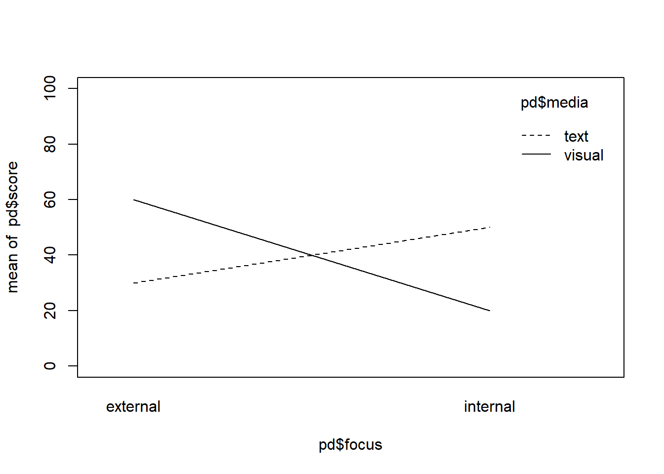
mean(pd$score[pd$focus == "internal"]) != mean(pd$score[pd$focus == "external"])## [1] TRUEmean(pd$score[pd$media == "text"]) == mean(pd$score[pd$media == "visual"])## [1] TRUEWe can see that the above situation satisfies all things that we wanted to specify:
- The means of the two focus groups are not the same so that internal are lower than external values if we pool over the media conditions.
- The mean for both media conditions are the same so there is no main-effect.
- The lines cross over showing the interaction that we wanted.
However, three problems remain here. First of all, the simple slope for the visual messages is steeper than the simple slope for the text messages, which is not something we specified in our hypotheses beforehand. It rather comes as a side-effect of that we want our internal means to be lower than the external means but we also want the visual messages to be more impactful in the internal condition while our text-messages should be more impactful on the external conditions. Do we find this plausible or do we think this would rather be the other way around?
This a good point for a short reflection: You might already be overwhelmed how complicated power-analysis by simulation already is with these still relatively simple designs. However, notice that e.g. the follow-up tests for the slopes are things that we can care about but we do not need to care about them. Our interaction-hypothesis is mainly interested in whether the difference in scores between the visual and the text messages when comparing the internal focus group is the same as the difference for the external groups. As this is clearly not the case in this example, we are good to go and test the interaction hypothesis. However, if we clearly are interested in the simple slopes and have hypotheses about them, we can put it in our simulation, and that of course urges us to think some more but it is a great tool to see whether we actually thought about everything, as this might be a point that would have slipped our attention entirely when running a classical power-analysis and pre-registering the overall interaction only. Now, we can think about it if we want to or continue by saying that for now we only want to specify the interaction.
Let us assume that we are fine with the fact that visual messages differ somewhat more than text messages. However, the numbers we have chosen so far are all but plausible. In this case, if we want to come up with more plausible numbers it is good if, instead of thinking about means directly, we make assumptions about how each of the group-means will differ from the overall population mean. For instance, we can assume in this case that all groups might actually have a more negative attitude towards smoking after seeing the text or visual message no matter whether they were externally and internally (ideally we would of course use a pre-post test design but lets keep that for later). Thus, we could for example assume that (having no better data on this) people are on average indifferent about smoking, therefore assuming the population mean is 50. Now lets see what this would imply in terms of change scores for the numbers above:
change_TI <- mean_TI-50
change_VI <- mean_VI-50
change_TE <- mean_TE-50
change_VE <- mean_VE-50

barplot(c(change_TI, change_VI, change_TE, change_VE), names.arg = c("TI", "VI", "TE", "VE"))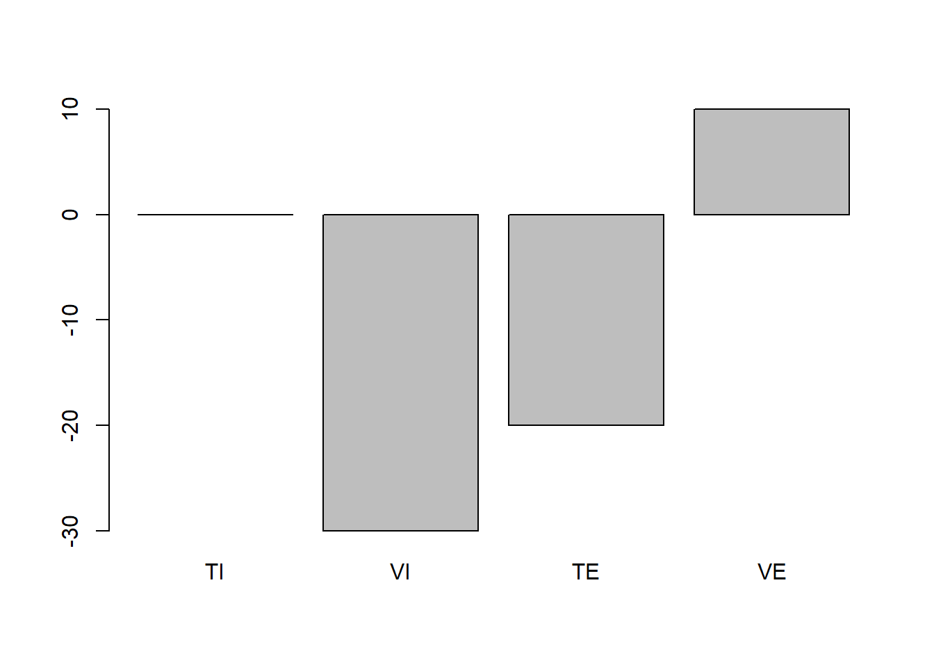
Thus, this does not seem entirely plausible. The VE group increases in their attitude towards cigarettes compared to the assumed population mean and the TI group does not change at all. This is not what we would expect. However, as we want to keep the rank-order of the bars the same (i.e. order of difference-magnitudes between the groups should stay the same as above) we will start with the highest bar here and adjust it to a position where it would actually make sense compared to the population mean. Lets assume that the looking at these external pictures would actually decrease the population mean of smoking attitude by 3 points on average. This is just a consequence of that I think an intervention of this would be rather weak as most people do not see these pictures for the first time and also might not be influences so much by looking at them to begin with. Thus my mean of group_VE becomes 47.
Next, when looking at the TI group, I think hat this group might decrease more strongly compared to the other group (it is internal), so the new mean after reading texts about yourself might be 45 in this case.
The next group is the TE group which should be lower than the other two groups before. However given that it is also an external group, and I expect internal messages to work better, it is probably not much stronger than the TI group, so I will assume the mean is 43.
Last, the strongest of the changes I would probably expect for the VI group so I can assume that the change might be 10 points in this case so that their mean will become 40.
Let us plot these new means again.
focus <- rep(c("internal", "external"), each = 2)
media <- rep(c("text", "visual"), times = 2)
mean_TI <- 43
mean_VI <- 40
mean_TE <- 45
mean_VE <- 47

pd <- data.frame(score = c(mean_TI, mean_VI, mean_TE, mean_VE), focus = focus, media = media)

interaction.plot(pd$focus, pd$media, pd$score, ylim = c(0,100))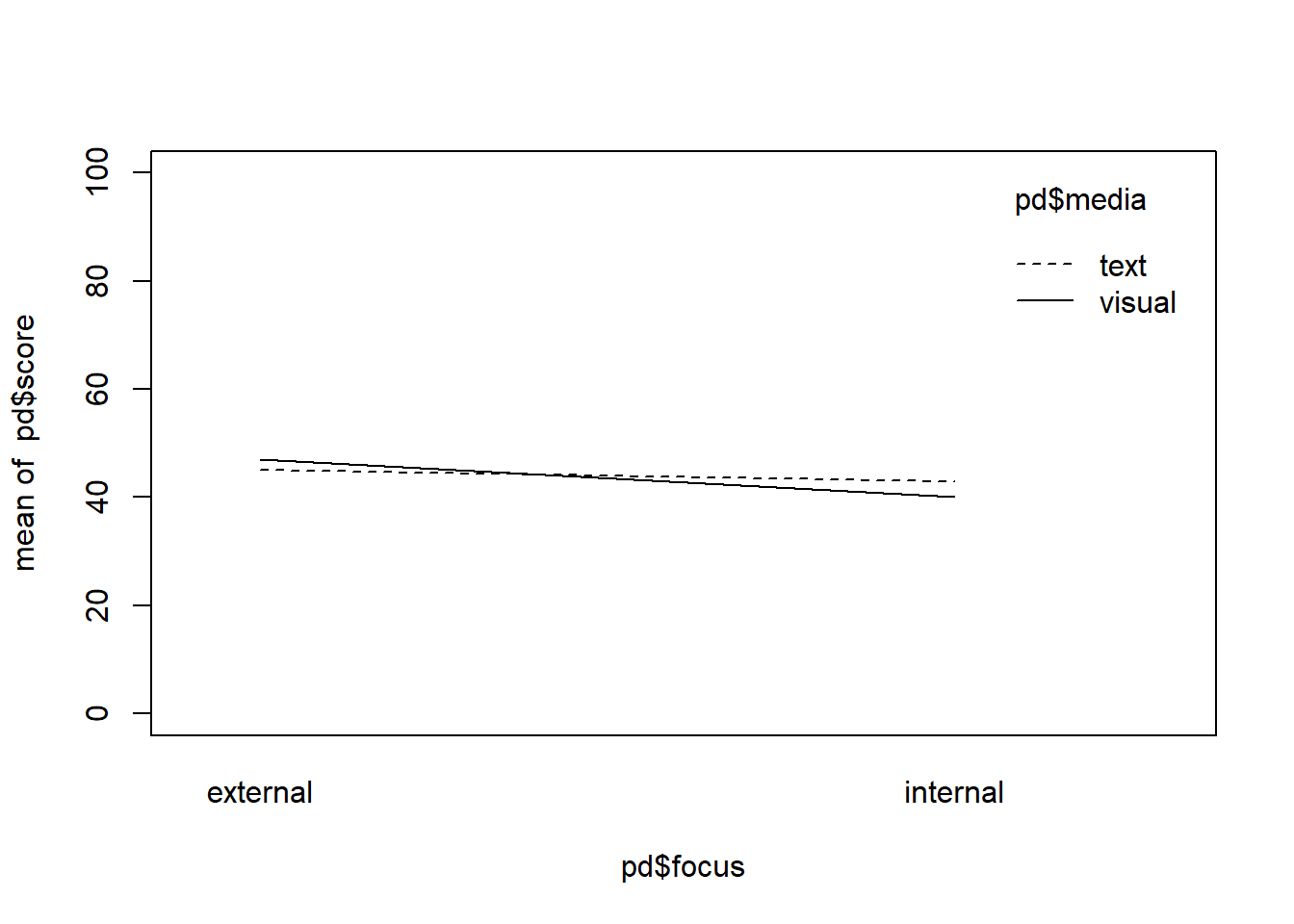
mean(pd$score[pd$focus == "internal"]) != mean(pd$score[pd$focus == "external"])## [1] TRUEmean(pd$score[pd$media == "text"]) == mean(pd$score[pd$media == "visual"])## [1] FALSENote that in this new example, technically there is a difference between the two media groups on average but it is only .50 points, so I would argue that it is small enough to represent our assumption of “no” effect, as in real-life “no” effect in terms of a difference being actually 0 is rather rare anyway.
Ok, so after rule-of-thumbing our way through all the different group-means, we have to consider what standard deviation we find plausible in this situation.
It is plausible, that the intervention that we are administering might not directly influence the spread in each group, so we might as well assume that the spread is the same in each group. What should we choose in this case? Let us think about the population. We said that people would in average be indifferent about smoking with a mean of 50 on a 100-point scale. How big should the spread on this scale be, i.e. between which values do we assume most people to be on this scale. It is probably likely that most people will not have a very good attitude about smoking, say 80 or higher. The lower end is more difficult to predict in this case, there might as well be more people that have a very negative opinion. In fact, the distribution might be skewed rather than symmetric, with more people having very negative opinions and a rather long tail. In any case, we will use this upper-limit assumption to come up with some reasonable standard-deviation. If we start at 50 and we want most people to be < 80, we can set the 2-SD bound at 80 to get a standard-deviation of 15 (80-50)/2. Thus let us assume that each of our groups has a standard-deviation of 15 points.
Thus our distributions that we would have are
group_TI = normal(n, 43, 15)
group_VI = normal(n, 40, 15)
group_TE = normal(n, 45, 15)
group_VE = normal(n, 47, 15)
With these groups we can now run an ANOVA.
Before getting into the power-analysis part lets just have a look what would happen if we had 10,000 people per group and would use this in our ANOVA.
First we will do this by using the aov_car function from the afex package.
## Loading required package: afex## Loading required package: lme4## Loading required package: Matrix## Registered S3 methods overwritten by 'car':
## method from
## influence.merMod lme4
## cooks.distance.influence.merMod lme4
## dfbeta.influence.merMod lme4
## dfbetas.influence.merMod lme4## ************
## Welcome to afex. For support visit: http://afex.singmann.science/## - Functions for ANOVAs: aov_car(), aov_ez(), and aov_4()
## - Methods for calculating p-values with mixed(): 'KR', 'S', 'LRT', and 'PB'
## - 'afex_aov' and 'mixed' objects can be passed to emmeans() for follow-up tests
## - NEWS: library('emmeans') now needs to be called explicitly!
## - Get and set global package options with: afex_options()
## - Set orthogonal sum-to-zero contrasts globally: set_sum_contrasts()
## - For example analyses see: browseVignettes("afex")
## ************##
## Attaching package: 'afex'## The following object is masked from 'package:lme4':
##
## lmerrequire(afex)n <- 1e5
group_TI <- rnorm(n, 43, 15)
group_VI <- rnorm(n, 40, 15)
group_TE <- rnorm(n, 45, 15)
group_VE <- rnorm(n, 47, 15)
participant <- c(1:(n*4))
focus <- rep(c("internal", "external"), each = n*2)
media <- rep(c("text", "visual"), each = n, times = 2)
aov_dat <- data.frame(participant = participant, focus = focus, media = media, score = c(group_TI, group_VI, group_TE, group_VE))
aov_car(score ~ focus*media+ Error(participant), data = aov_dat, type = 3)## Contrasts set to contr.sum for the following variables: focus, media## Anova Table (Type 3 tests)
##
## Response: score
## Effect df MSE F ges p.value
## 1 focus 1, 399996 225.28 8811.28 *** .02 <.0001
## 2 media 1, 399996 225.28 126.75 *** .0003 <.0001
## 3 focus:media 1, 399996 225.28 2703.27 *** .007 <.0001
## ---
## Signif. codes: 0 '***' 0.001 '**' 0.01 '*' 0.05 '+' 0.1 ' ' 1We see that, if we collect 10,000 people per group, everything would be significant with focus having the biggest effect (look at the ges column in the table for generalized eta-squared values) and with media having the smallest effect (in fact close to 0 as we wanted).
That even the main-effect for media is still significant just shows that this happens even with very small deviations from the exact null-hypothesis in these huge samples.
Note that again we could rewrite this anova as a dummy-coded linear model as:
\[ score_i = \beta_0 + \beta_1X_1 + \beta_2X_2 + \beta_3X_1X_2 \]
By making dummy-variables we can code this in lm
aov_dat$focus_dummy <- ifelse(aov_dat$focus == "internal", 0 , 1)
aov_dat$media_dummy <- ifelse(aov_dat$media == "text", 0 , 1)

lm_int <- lm(score ~ 1 + focus_dummy + media_dummy + focus_dummy:media_dummy, data = aov_dat)
From the estimates that we get here we see how the model is estimated:
\(\beta_0\) = mean(group_TI) as both dummies are 0 for this one.
\(\beta_1\) = mean(group_TE)-mean(group_TI) as the focus variable changes from 0 to 1 within the text-group
\(\beta_2\) = mean(group_VI)-mean(group_TI) as the media variable changes from 0 to 1 within the internal focus group
\(\beta_3\) = mean(group_VE)-mean(group_TE)+mean(group_TI)-mean(group_VI) to see what a crossover of the variables (i.e. the interaction) compares to \(\beta_0\)
If we want to test whether the effect of the interaction, for instance is significant, we can conduct an ANOVA for the interaction to see how the model with the interaction compares to a model without the interaction, which we do in the following code-block by fitting a model that does not have the interaction in their and compare it with the anova function.
lm_null <- lm(score ~ 1 + focus_dummy + media_dummy, data = aov_dat)
anova(lm_null, lm_int)
## Analysis of Variance Table
##
## Model 1: score ~ 1 + focus_dummy + media_dummy
## Model 2: score ~ 1 + focus_dummy + media_dummy + focus_dummy:media_dummy
## Res.Df RSS Df Sum of Sq F Pr(>F)
## 1 399997 90721027
## 2 399996 90112027 1 609000 2703.3 < 2.2e-16 ***
## ---
## Signif. codes: 0 '***' 0.001 '**' 0.01 '*' 0.05 '.' 0.1 ' ' 1Again, we find the same F-value and p-value as before, which should not be surprising considering we did the same test.
I will leave it to you which of the two methods, i.e. using the regular aov functions or specifying linear models, you prefer.
An obvious advantage of the aov function is that we do not have to specify nested models but it is also sort of a black-box approach, while in the linear models, we get estimated effects and can see whether the model does actually behaves as we would expect.
Quick detour: Contrast Coding and Centering
Going back to the aov_car output above, you might have noticed that the function informed us that it set [contrasts] to contr.sum for the following variables: focus, media.
What does this mean?
It means that instead of using dummy-coding as we did when we created the dummy variables, it instead assigned a -1 to a level of the variable while setting a 1 to the other level.
We can check what this looks like if we set it manually to the variables in the data-set.
aov_dat$media_sum <- factor(aov_dat$media)
contrasts(aov_dat$media_sum) <- contr.sum(2)
contrasts(aov_dat$media_sum)
## [,1]
## text 1
## visual -1aov_dat$focus_sum <- factor(aov_dat$focus)
contrasts(aov_dat$focus_sum) <- contr.sum(2)
contrasts(aov_dat$focus_sum)## [,1]
## external 1
## internal -1If we compare this to our dummy variables:
media:
- text = 0
- visual = 1
focus:
- internal = 0
- external = 1
Let’s re-run the linear model with these variables and see what we get.
aov_dat$media_sum_num <- ifelse(aov_dat$media == "text", 1, -1)
aov_dat$focus_sum_num <- ifelse(aov_dat$focus == "external", 1, -1)

lm_int_sum <- lm(score ~ 1 + focus_sum_num + media_sum_num + focus_sum_num:media_sum_num, data = aov_dat)
lm_int_sum
##
## Call:
## lm(formula = score ~ 1 + focus_sum_num + media_sum_num + focus_sum_num:media_sum_num,
## data = aov_dat)
##
## Coefficients:
## (Intercept) focus_sum_num
## 43.7756 2.2277
## media_sum_num focus_sum_num:media_sum_num
## 0.2672 -1.2339lm_null_sum <- lm(score ~ 1 + focus_sum_num + media_sum_num, data = aov_dat)
lm_null_sum##
## Call:
## lm(formula = score ~ 1 + focus_sum_num + media_sum_num, data = aov_dat)
##
## Coefficients:
## (Intercept) focus_sum_num media_sum_num
## 43.7756 2.2277 0.2672anova(lm_null_sum,lm_int_sum)## Analysis of Variance Table
##
## Model 1: score ~ 1 + focus_sum_num + media_sum_num
## Model 2: score ~ 1 + focus_sum_num + media_sum_num + focus_sum_num:media_sum_num
## Res.Df RSS Df Sum of Sq F Pr(>F)
## 1 399997 90721027
## 2 399996 90112027 1 609000 2703.3 < 2.2e-16 ***
## ---
## Signif. codes: 0 '***' 0.001 '**' 0.01 '*' 0.05 '.' 0.1 ' ' 1We see immediately that the estimates changed somewhat. Now, for example the intercept represents the mean of all 4 other means (i.e. the grand mean):
mean(c(mean(group_TI), mean(group_TE), mean(group_VE), mean(group_VI))) = 43.775609.
and the first estimate represents the difference of each focus level from that grand-mean, for the “internal groups this is”
mean(c(mean(group_TI), mean(group_VI)))-mean(c(mean(group_TI), mean(group_TE), mean(group_VE), mean(group_VI))) = -2.2276811
and for the external groups this is
mean(c(mean(group_TE), mean(group_VE)))-mean(c(mean(group_TI), mean(group_TE), mean(group_VE), mean(group_VI))) = 2.2276811
respectively.
Why would we use this coding-scheme in the linear model instead of the other one? The p-value for the interaction is exactly the same in both cases. However, if we compare the p-values of main-effects here, we will see how they differ.
For instance, if we tell aov_car that we want to keep our dummy-coding instead of changing it, we can see how the two outputs differ.
aov_car(score ~ focus*media+ Error(participant), data = aov_dat, type = 3, afex_options("check_contrasts" = FALSE))## Anova Table (Type 3 tests)
##
## Response: score
## Effect df MSE F ges p.value
## 1 focus 1, 399996 225.28 876.77 *** .002 <.0001
## 2 media 1, 399996 225.28 829.66 *** .002 <.0001
## 3 focus:media 1, 399996 225.28 2703.27 *** .007 <.0001
## ---
## Signif. codes: 0 '***' 0.001 '**' 0.01 '*' 0.05 '+' 0.1 ' ' 1As you can see, these results are a bit weird, as we seem to have the same effect-size for both main-effects, but did we not simulate a much bigger effect of focus compared to media1? Something seems to be off here. This has to do with the fact that in classical dummy-coding (also called treatment coding) you cannot easily test main-effects when interactions are present in the model. For the interaction on the other hand it does not matter. You can read more about this in this blog post by Dale Barr but the take-home message here is that, whenever we have an interaction in our model, we want to use sum-to-zero coding rather than dummy-coding. This is why the results of the last anova do not show the behavior that we simulated.
Thus, for the rest of the tutorial we will use sum-to-zero contrasts coding.
Running the power-analysis
I will use the lm way here as it is much faster (about 8 times faster in a quick test) than the aov_car method.
To track our power, we can directly extract p-values from the anova object, just as we did for the t.test objects earlier.
The only thing that we still need to do is specify our test criteria. Imagine that this time we are hired by the government and are asked to evaluate which of the health-warnings on cigarette packages would work best in which of the situations that we investigate. They gave us a lot of money to do this, but they do not want to draw any conclusions that are unwarranted as implementing new laws costs a lot of money. Thus, we want to set our alpha-level quite conservatively at \(\alpha = .001\) to only make a non-warranted claim about the interaction effect in 1 of every 1,000 experiments. Moreover, we also want to be sure that we actually detect an effect and therefore want to keep our power high at 95% to be sure that if there is an interaction we would detect it in 19 out of 20 cases.
Now we have everything that we need to set up the code-chunk below to run a power-analysis similar to the ones we have been running previously, just this time with an ANOVA coded as a linear model. If we would again try out every sample-size, this would take a very long time until we reach our power criterion and we would probably still be sitting here tomorrow or the day after. In these cases, it makes sense to run a two-stage power analysis in which we, in the first stage, try out various sample-sizes with a very low resolution (e.g. n = 10, n = 100, n = 200) etc. to get a rough idea of where we can expect our loop to end. Afterwards, we will increase the resolution to find how many participants exactly we would need. The first step with the low resolution is performed below.
set.seed(1)
n_sims <- 1000 # we want 1000 simulations
p_vals <- c()
power_at_n <- c(0) # this vector will contain the power for each sample-size (it needs the initial 0 for the while-loop to work)
n <- 100 # sample-size and start at 100 as we can be pretty sure this will not suffice for such a small effect
n_increase <- 100 # by which stepsize should n be increased
i <- 2

power_crit <- .95
alpha <- .001

while(power_at_n[i-1] < power_crit){
  for(sim in 1:n_sims){
    group_TI <-  rnorm(n, 43, 15)
    group_VI <-  rnorm(n, 40, 15)
    group_TE <-  rnorm(n, 45, 15)
    group_VE <-  rnorm(n, 47, 15)

    participant <- c(1:(n*4))
    focus <- rep(c("internal", "external"), each = n*2)
    media <- rep(c("text", "visual"), each = n, times = 2)

    aov_dat <- data.frame(participant = participant, focus = focus, media = media, score = c(group_TI, group_VI, group_TE, group_VE))
    aov_dat$media_sum_num <- ifelse(aov_dat$media == "text", 1, -1) # apply sum-to-zero coding
    aov_dat$focus_sum_num <- ifelse(aov_dat$focus == "external", 1, -1)
    lm_int <- lm(score ~ 1 + focus_sum_num + media_sum_num + focus_sum_num:media_sum_num, data = aov_dat) # fit the model with the interaction
    lm_null <- lm(score ~ 1 + focus_sum_num + media_sum_num, data = aov_dat) # fit the model without the interaction
    p_vals[sim] <- anova(lm_int, lm_null)$`Pr(>F)`[2] # put the p-values in a list
  }
    print(n)
    power_at_n[i] <- mean(p_vals < alpha) # check power (i.e. proportion of p-values that are smaller than alpha-level of .10)
    names(power_at_n)[i] <- n
    n <- n+n_increase # increase sample-size by 100 for low-resolution testing first
    i <- i+1 # increase index of the while-loop by 1 to save power and cohens d to vector
}
## [1] 100
## [1] 200
## [1] 300
## [1] 400
## [1] 500
## [1] 600
## [1] 700
## [1] 800
## [1] 900power_at_n <- power_at_n[-1] # delete first 0 from the vectorplot(as.numeric(names(power_at_n)), power_at_n, xlab = "Number of participants per group", ylab = "Power", ylim = c(0,1), axes = TRUE)
abline(h = .95, col = "red")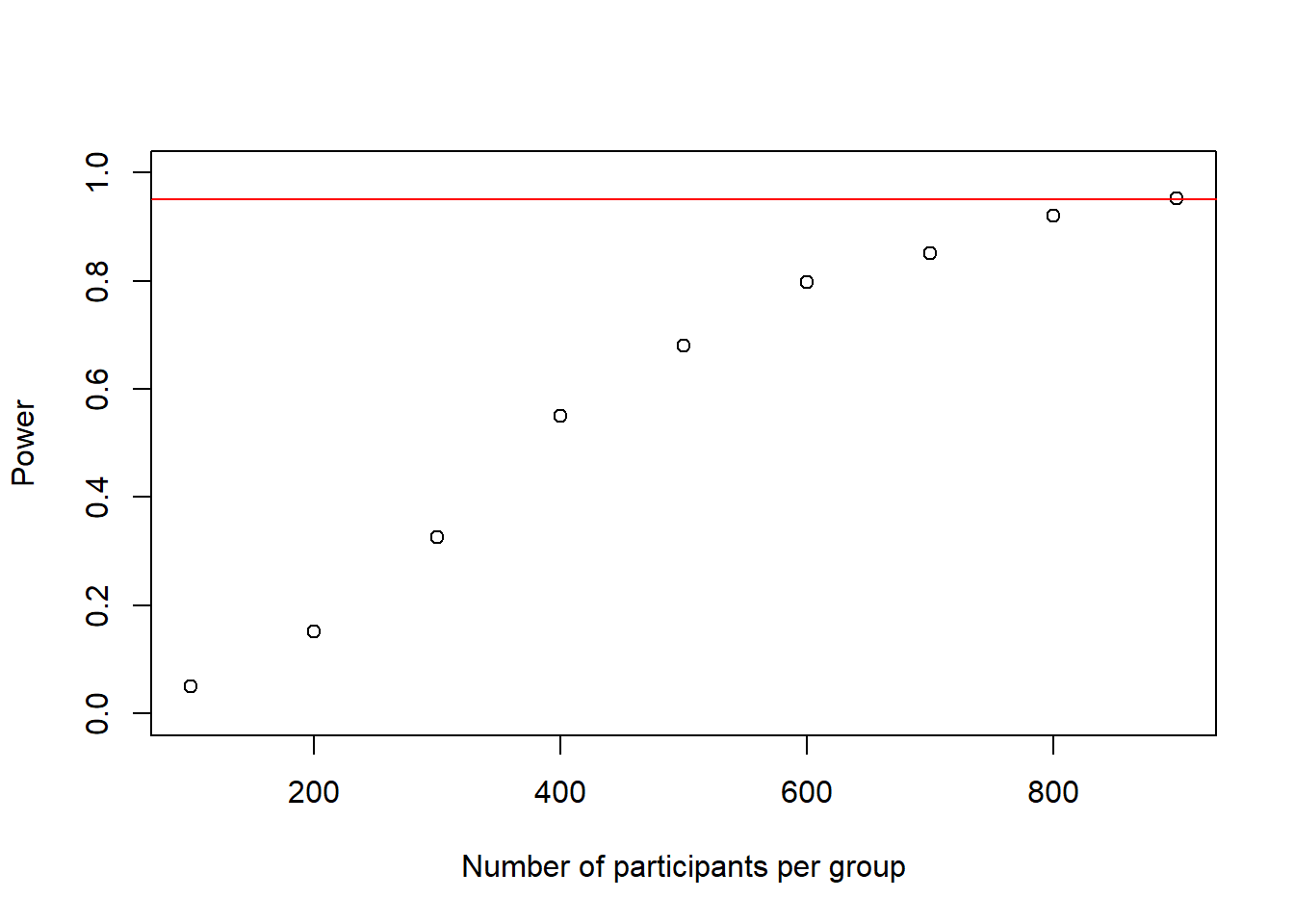
We see that at roughly 900 participants our loop ran into a situation where we have sufficient power. Thank god we did not do this 1-by-1. Now we can have a closer look at sample-sizes between 800 and 900. Probably, at this sample-size it does not really matter whether we calculate +/- 10 participants in terms of budget, so we can start at 800 and increase in steps of 10 and instead increase the simulation-number per sample-size to 10,000 to get even more precise results for each particular sample-size, as this is a rather important power-analysis impact-wise. Afterwards, if we really wanted to we could of course run a third round between the last two 10-people cutoffs and increase the sample-size by 1 to reach an exact sample-size.
set.seed(1)
n_sims <- 10000 # we want 10000 simulations
p_vals <- c()
power_at_n <- c(0) # this vector will contain the power for each sample-size (it needs the initial 0 for the while-loop to work)
delta_r2s<- c()
delta_r2s_at_n <- c(0)
n <- 800 # sample-size and start at 800 as we can be pretty sure this will not suffice for such a small effect
n_increase <- 10 # by which stepsize should n be increased
i <- 2
power_crit <- .95
alpha <- .001
while(power_at_n[i-1] < power_crit){
for(sim in 1:n_sims){
group_TI <- rnorm(n, 43, 15)
group_VI <- rnorm(n, 40, 15)
group_TE <- rnorm(n, 45, 15)
group_VE <- rnorm(n, 47, 15)
participant <- c(1:(n*4))
focus <- rep(c("internal", "external"), each = n*2)
media <- rep(c("text", "visual"), each = n, times = 2)
aov_dat <- data.frame(participant = participant, focus = focus, media = media, score = c(group_TI, group_VI, group_TE, group_VE))
aov_dat$media_sum_num <- ifelse(aov_dat$media == "text", 1, -1)
aov_dat$focus_sum_num <- ifelse(aov_dat$focus == "external", 1, -1)
lm_int <- lm(score ~ 1 + focus_sum_num + media_sum_num + focus_sum_num:media_sum_num, data = aov_dat)
lm_null <- lm(score ~ 1 + focus_sum_num + media_sum_num, data = aov_dat)
p_vals[sim] <- anova(lm_null, lm_int)$`Pr(>F)`[2]
delta_r2s[sim]<- summary(lm_int)$adj.r.squared-summary(lm_null)$adj.r.squared
}
print(n)
power_at_n[i] <- mean(p_vals < alpha) # check power (i.e. proportion of p-values that are smaller than alpha-level of .10)
delta_r2s_at_n[i] <- mean(delta_r2s)
names(power_at_n)[i] <- n
names(delta_r2s_at_n)[i] <- n
n <- n+n_increase # increase sample-size by 100 for low-resolution testing first
i <- i+1 # increase index of the while-loop by 1 to save power and cohens d to vector
}## [1] 800
## [1] 810
## [1] 820
## [1] 830
## [1] 840
## [1] 850
## [1] 860
## [1] 870
## [1] 880
## [1] 890power_at_n <- power_at_n[-1] # delete first 0 from the vector
delta_r2s_at_n <- delta_r2s_at_n[-1] # delete first 0 from the vectorAs you will notice when you run this yourself, this simulation already takes quite some time. Later, when we work with mixed models in part IV, we will see how we can run such a simulation on multiple processor-cores simultaneously to solve this problem to at least some extent.
plot(as.numeric(names(power_at_n)), power_at_n, xlab = "Number of participants per group", ylab = "Power", ylim = c(0,1), axes = TRUE)
abline(h = .95, col = "red")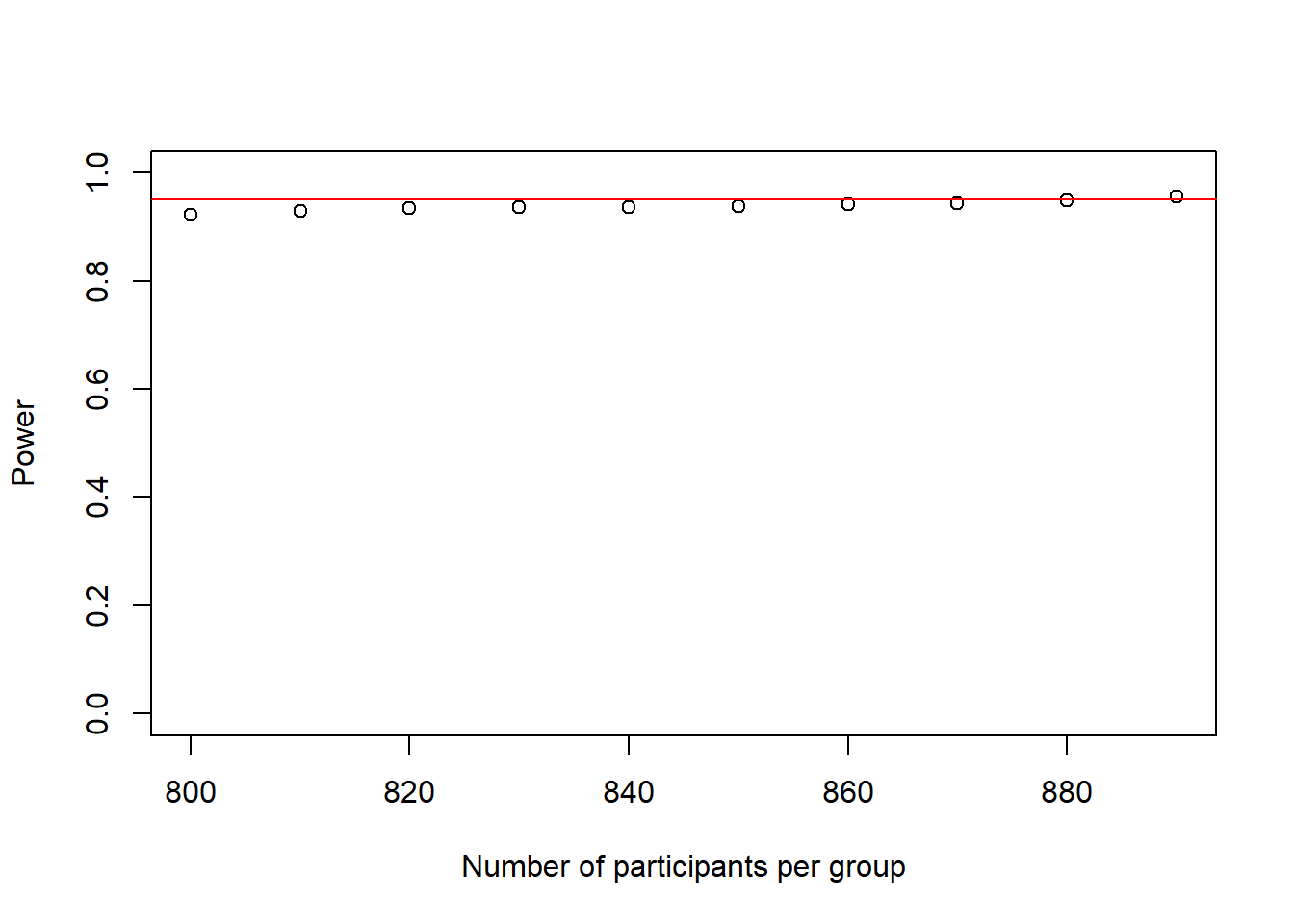
This power-curve looks a bit odd, as it looks almost flat. What this shows however, is that power is not increasing linearly but tends to increase faster at the beginning and slower towards reaching 1.
In any case, 890 people per group would be enough to reach our desired power of .95.
Note how close this is to the 900 from our low-resolution simulation above, showing the merits of this approach.
Also note that the change in amount of variance explained \(\Delta R^2\) only increases by about delta_r2s_at_n[length(delta_r2s_at_n)] = 0.0067977.
Whether this ~0.6% is a meaningful amount of added variance explained to begin with and whether it is worth spending money in order to test about 3,500 people without even knowing what this attitude measure in this case even tells us in terms of smoking-behavior is a whole other question and cannot be answered with power-analysis (probably the answer would be that it is not so important though).
Adding a Numeric Predictor
In this last bit of part III of this tutorial I want to demonstrate how we can add numeric predictors to our models as, so far, we only worked with factors. Again, knowing how to re-specify an ANOVA as a linear model is helpful in this case if we have both, factorial and numerical predictors.
We could also assume that the effect that our predictors have depend on other factors. For example, we could think that the more cigarettes a person smokes each day, the less effective any treatment would be independent of what strategy we would use. Thus, if we assume that the aforementioned effect-sizes would be the expected value for a non-smoking population, including smokers would make this effect less pronounced. In other words, the more a person smokes, the smaller the expected effect size for that person should be.
How do we do this? If we reformulate our problem above we could say that if a person smokes 0 cigarettes a day she should get 100% of the expected effect (e.g. the decrease of 7 points in the internal text-group). Now, we can take the maximum amount of cigarettes that we think a person can smoke per day (or what we expect the 95% CI to be in a smoking population for instance). Let us say we assume this to be 36 cigarettes a day (about 2 packages). Now if we want a person that smokes 0 cigarettes to get the full 7 points and a person who smokes 36 cigarettes to get 0 percent of the effect, we can rewrite the effect like this
\[y{_i} = \bar y \times \frac{max_{n}-n}{max_n}\]
or if we fill in the numbers for a non-smoker:
\[y{_i} = 7 \times \frac{36-0}{36} = 7\]
and someone who smokes 14 cigarettes a day:
\[y{_i} = 7 \times \frac{36-14}{36} = 5.64\]
Thus, our effect of 7 points now depends on how much someone smokes.
Now we have to come up with an assumption of how much people smoke in the population. A quick google search can tell us that, in the Netherlands, 23.1% of adults smoke. We can also find that people who smoke consume ca. 11 cigarettes on average. Thus, we will make a population in which 76.9 percent of the people do not smoke and 23.1 percent smokes 11 cigarettes on average. For the cigarette count in the smoking population we will choose a Poisson distribution, as it is often a good representation of count-data like this.
You might never have heard of a Poisson distribution and to avoid confusion here: We could just use a uniform distribution between 1 and 36 for example so that smoking 30 cigarettes a day is just as likely as smoking 1 cigarette, given that a person is a smoker. However, I do not think that this is the case and that the likelihood of a smoker smoking 30 cigarettes is smaller compared to only smoking 5 cigarettes. The Poisson distribution mainly carries this assumption forward into the simulation. As you continue simulating stuff in the future, you will probably get to know more of these useful distributions that neatly describe certain assumptions that we have about the data.
To create a population like this we can do the following:
n <- 1000# sample size

smoke_yes_no <- ifelse(runif(n, 0, 100) < 77, 0, 1) # vector telling us whether each "person" smokes or not

n_smoke <- c() # vector that will contain number of cigarettes per day smoked by each person

# create the number of smoked cigarettes
for(i in 1:length(smoke_yes_no)){
  if(smoke_yes_no[i] == 1){
    n_smoke[i] <- rpois(1,11) # simulate 1 cigarette count from a poisson distribution with mean 11
  } else{
    n_smoke[i] <- 0}
}
In the above code we check for each person whether they are a smoker or not and if so, say that the person’s number of cigarettes smoked comes from a Poisson distribution or otherwise it will be 0 by definition.
To implement this for each group, we can just replace the means of the groups by this formula:
set.seed(1234)
group_TI <-  rnorm(n, (50-(7*((max(n_smoke)-n_smoke)/max(n_smoke)))), 15)
group_VI <-  rnorm(n, (50-(10*((max(n_smoke)-n_smoke)/max(n_smoke)))), 15)
group_TE <-  rnorm(n, (50-(5*((max(n_smoke)-n_smoke)/max(n_smoke)))), 15)
group_VE <-  rnorm(n, (50-(3*((max(n_smoke)-n_smoke)/max(n_smoke)))), 15)

participant <- c(1:(n*4))
focus <- rep(c("internal", "external"), each = n*2)
media <- rep(c("text", "visual"), each = n, times = 2)

aov_dat <- data.frame(participant = participant, focus = focus, media = media, score = c(group_TI, group_VI, group_TE, group_VE))

aov_dat$media_sum_num <- ifelse(aov_dat$media == "text", 1, -1)
aov_dat$focus_sum_num <- ifelse(aov_dat$focus == "external", 1, -1)
aov_dat$n_smoke <- rep(scale(n_smoke))

lm_int <- lm(score ~ 1 + focus_sum_num * media_sum_num * n_smoke, data = aov_dat)
summary(lm_int)
##
## Call:
## lm(formula = score ~ 1 + focus_sum_num * media_sum_num * n_smoke,
## data = aov_dat)
##
## Residuals:
## Min 1Q Median 3Q Max
## -50.287 -10.129 0.189 9.930 48.593
##
## Coefficients:
## Estimate Std. Error t value
## (Intercept) 44.44569 0.23621 188.160
## focus_sum_num 2.12720 0.23621 9.005
## media_sum_num 0.21372 0.23621 0.905
## n_smoke 1.77929 0.23633 7.529
## focus_sum_num:media_sum_num -0.81755 0.23621 -3.461
## focus_sum_num:n_smoke -0.27972 0.23633 -1.184
## media_sum_num:n_smoke -0.10452 0.23633 -0.442
## focus_sum_num:media_sum_num:n_smoke 0.06719 0.23633 0.284
## Pr(>|t|)
## (Intercept) < 2e-16 ***
## focus_sum_num < 2e-16 ***
## media_sum_num 0.365634
## n_smoke 0.0000000000000629 ***
## focus_sum_num:media_sum_num 0.000544 ***
## focus_sum_num:n_smoke 0.236651
## media_sum_num:n_smoke 0.658334
## focus_sum_num:media_sum_num:n_smoke 0.776180
## ---
## Signif. codes: 0 '***' 0.001 '**' 0.01 '*' 0.05 '.' 0.1 ' ' 1
##
## Residual standard error: 14.94 on 3992 degrees of freedom
## Multiple R-squared: 0.03674, Adjusted R-squared: 0.03505
## F-statistic: 21.75 on 7 and 3992 DF, p-value: < 2.2e-16Note how the effects that we put in before are still there but they are weaker now as we have smokers included in our sample. Moreover, smoking causes a more positive attitude towards smoking, just as we wanted, and the interaction between media and focus is not influenced by whether someone smokes or not, as we put the same punishment for the treatment effect in all the groups, leaving the interaction uninfluenced by whether someone smokes or not.
Summary
So now we have seen how we can simulate data for analyses that many people use in their everyday life as a (psychological) researcher. So far, all of the power-analyses that we did can also be done in standard software like G*Power (though in part I of this tutorial I explained why I still prefer simulation). However, as nice as these analyses are, we often deal with more complicated situations where we have to deal with hierarchical or cross-classified data. In these cases, other approaches like linear-mixed effects models, also called hierarchical models, need to be used to analyse our data. This is where simulation really shines as the structure of the data strongly depends on the research design and in a point-and-click software (though existing) it is difficult to offer all the flexibility that we might need. Thus, in the fourth part, we will see how we can simulate data and run a power-analysis in these cases.
Footnotes
We can actually see that this is the case by calculating cohens d for both assuming that we would perform a t-test for each of the 2 factors with the between-subject cohens d formula from part II of this tutorial: focus:
(mean(aov_dat$score[aov_dat$focus == "internal"])-mean(aov_dat$score[aov_dat$focus == "external"]))/sqrt((sd(aov_dat$score[aov_dat$focus == "internal"])^2+sd(aov_dat$score[aov_dat$focus == "external"])^2)/2)= -0.2824849 media:(mean(aov_dat$score[aov_dat$media == "text"])-mean(aov_dat$score[aov_dat$media == "visual"]))/sqrt((sd(aov_dat$score[aov_dat$media == "text"])^2+sd(aov_dat$score[aov_dat$media == "visual"])^2)/2)= 0.0281052↩︎