Power Analysis by Data Simulation in R - Part IV
August 5, 2020
Power Analysis by simulation in R for really any design - Part IV
This is the final part of my Power Analysis in R series, focusing on (Generalized) Linear Mixed Effects Models. I assume that, at this point, you already read Parts I to III of this tutorial, if you haven’t I suggest doing so before working through this. As I already mentioned in previous parts, there are good available options for Mixed Model power analysis already, an overview of which can be found in the SOP document of the D2P2 lab. This tutorial however, is meant to give you a deeper understanding of what you are doing when you simulate data and do power analysis by simulation. I hope that the last 3 parts already helped you in achieving this and that this final part will help to generalize this knowledge to mixed-effects models. The good news is that we will actually not be doing a lot of new stuff, the novel part about mixed-effects models compared to the models that we simulated in part III is mostly that we need to use the same methods and add some new things to them (after all this tutorial is about teaching a general skill so it’s good that we can build up on what we learned in the first three parts). Still, there is a lot of ground to cover so we better get started right away.
Mixed-effects models are extremely powerful in that they are incredibly flexible to the data-structure that they can work with, most notably that they:
- They are able to handle between-subject and within-subject effects in the same model along with numeric predictors (covariates).
- They allow for non-independent observations, i.e. observations from the same unit of measurement (e.g. a participant, a school, a country etc.) and even from multiple nested or crossed (see infobox below) units of measurements simultaneously.
A few words on nested vs. crossed random effects
As mixed-effects model literature has unfortunately developed to use different terms to mean different things, I just want to spend a few words on what I mean by nested as opposed to crossed random effects.
A data structure is nested when observations are organized in one or more clusters. The classic example of nested data is that we observe the performance of school-children over time. Because we collect data throughout multiple years, we have multiple observations per child, so we can say that observations are nested within children. We also observe multiple children per class, so children are nested within classes. If we involve not one but multiple schools in our study, then we have children nested in classes nested in schools. If we have schools from multiple countries we have …. well, you get the idea. It is important to realize that nested data is defined by “belong” and “contain” relationships. The data is fully nested if (per reasonable assumption in this case) each child only belongs to one specific class, each class only belongs to one school etc. This point is sometimes confusing as we might, in our data-frame, have multiple classes from different schools that have the same ID in the data-set, for instance there might be a class called 9A in schools 1 and 2. However, it is important to realize that these classes are not the same but different classes in reality. They contain different students and belong to a different school. Therefore the data is nested.
In crossed, or cross-classified data, each observation does also belong to not only 1, but multiple nesting levels. However, the as opposed to fully nested data, the nesting levels are not bounded to each other by a “contain” or “belong” relationship as was the case in the example above where classes contained students and belonged to schools. A classic example of cross-classified data is experimental data in which, for instance, people had to press a button quickly whenever pictures appear on a computer screen. Imagine that we recruit 100 participants and each sees the same 20 pictures 5 times. In this case we have 100x20x5 = 10,000 observations. Imagine we would identify these observations by their row-number (i.e. 1 … 10,000). Now each of these observations “belongs” to a participant, and “belongs” to a specific stimulus. For instance, assuming that the data is ordered ascending by participant and stimulus, the first observation (observation 1) belongs to participant 1 and stimulus 1, the last observation (observation 10,000) belongs to participant 100 and stimulus 20. As you might already realize, in this case it is not the case that a participant either contains or belongs to a specific stimulus and vice versa: Each participant sees each stimulus, or framed differently, each stimulus presents itself to each participant - the two nesting levels are independent from each other, they are cross-classified.
Building up mixed-effects models
We will approach the simulation of mixed-effects models in a bottom-up approach. We will first start simple with a model that has only a single effect and nesting level and then explore different situations in which there are more fixed and random effects and both. Throughout this tutorial, we will use a new hypothetical research question focused on music preference. The overarching research goal will be to - once and for all - find out whether Rock or Pop music is better. Of course, we could just ask people what they prefer, but we do not want to do that because we want a more objective measure of what is Rock and Pop (people might have different ideas about the genres). Therefore, we will have participants listen to a bunch of different songs that are either from a Spotify “best-of-pop” or “best-of-rock” playlist and have them rate the song on a evaluation scale from 0-100 points. We will start this of really simple and make this design more complex along the way to demonstrate the different aspects that we need to consider when simulating mixed-model data.
Simulating a Within-Subject Effect
As a first demonstration, we will simulate a MEM with only the within-subject effect.
We also will now write a function that allows us to, quite flexibly, simulate various data structures.
No worries, it will make use of things that we already introduced in earlier parts of this tutorial (e.g. rnorm and mvrnorm) so you will hopefully be able to understand what is going on just fine.
To investigate the question stated above, we can use the following design:
- DV : liking of Song (0-100)
- IV (within-subject) : Genre of Song (Rock/Pop)
Note that we made the design choice that genre will be a within-subject effect. In theory, it could also be a between-subject design where a person listens to only 1 genre, pop or rock, but a within-subject design has the advantage that general liking of music across conditions (e.g. person 1 might like both genres more than person 2) does not affect the results (as much) as it would in a between-subject design.
I say “as much” because it could still affect the results even in a within subject design if, for instance, a person that likes music generally more will also show fewer difference between conditions compared to a person that dislikes music more generally. In that case, the overall score is related to the difference score which can impact our inference.
The first thing that we need to do is not entirely new for us at this point.
We will use the rnorm function to generate the scores for the 2 conditions.
However, we will now follow a slightly different approach where we will not create the 2 groups’ scores directly (i.e. use rnorm() for each group separately), but will instead only generate the design matrix of the data, i.e. the structure of the data without having any actual scores for the dependent variable in there.
Eventually we will then add the DV in a second step by calculating it’s value for each row in the data-set based on the values for the other variables in that row.
However, before we will use the “old” approach one last time because it allows us to explore some important insights.
Generating a design-matrix with 1 within-subject factor
As this is the first time we actually write a custom function in this tutorial, I will spend some time to explain.
The following function generate_design will allow us to pass any number of subjects that we would like it to generate.
In the function header, we pass the number of participants n_participants and the number of genres n_genres that our design should have.
Moreover it allows us to specify the number of songs per genre n_songs which at this part does not do anything in the function (we will add this functionality in a minute).
The function then calls expand.grid, a built-in R-function, that will do nothing but create one row in our data-frame for each possible combination of participant-number and genre.
The final line of the function returns this created design matrix whenever we call on the function.
generate_design <- function(n_participants, n_genres, n_songs){

  design_matrix <- expand.grid(participant = 1:n_participants, genre = 1:n_genres) # here we create the data-frame
  design_matrix$genre <- ifelse(design_matrix$genre ==1, "rock", "pop") # we rename the genres so its easier to follow (this is not really necessary)
  return(design_matrix) # return the data-frame
}
Lets start slow and first create a data-frame that represents 10 people listening to one song from each genre. Thus, when we have 10 people and 2 genres with 1 song each, there should be 20 rows in our data-frame. Let’s see
data1 <- generate_design(n_participants = 10, n_genres = 2, n_songs = 1)
paged_table(data1)
Nice! Indeed our data has 20 rows, and each participant listens to rock and pop once - exactly what we wanted.
Now, as said, we would like to have each person listen to more songs - lets say 20 songs per genre.
The first instinct here could be to add n_songs to the function just as we did add n_genre.
However, this does not work as songs are unique per genre.
That is, while each participant listens to both genres, each song only belongs to one genre.
For instance the specific song “Blank Space by Taylor Swift” only belongs to the “pop” but not the “rock” condition.
Thus, we need to make sure that the songs will have unique identifiers, rather than numbers that will appear in both conditions.
Luckily we can easily fix this:
generate_design <- function(n_participants, n_genres, n_songs){


  design_matrix <- expand.grid(participant = 1:n_participants, genre = 1:n_genres, song = 1:n_songs) # adding song to expand.grid
  design_matrix$genre <- ifelse(design_matrix$genre ==1, "rock", "pop")
  design_matrix$song <- paste0(design_matrix$genre, "_", design_matrix$song)
  return(design_matrix)
}
As you can see, we just added a slight modification to the function.
We added the song variable to expand.grid and in line 3 of the function we rename the song variable using paste0, a function that will just concatenate strings together.
We use this to create song-names that now include the genre name.
This way, song 1 in the rock-genre will have a different name from song 1 in the pop-genre, telling our model that these are in fact unique songs that cannot be interchanged.
Note that this also means that we will pass the number of songs per genre instead of the total number of songs.
Lets try this out.
If our code functions correctly, we should have 10 participants x2 genres x20 songs per genre = 400 rows in our data frame.
data2 <- generate_design(n_participants = 10, n_genres = 2, n_songs = 20) # note that we pass the number of songs per GENRE
data2 <- data2[order(data2$participant),] # order the data by participant number so its easier to see how its structured
paged_table(data2)
Indeed, we get 400 rows and each participant listens to 20 rock songs and 20 pop songs, that all have unique names - neat! Now that we have the design-simulation out of the way, let us give scores to the songs. We first will do this with only 1 song per person per genre (that is the same across participants) to keep the model simple first.
Revisiting the old simulation approach once more
As mentioned our DV is the liking of songs on a 100-point scale.
Let us assume that, in the population, both genres are liked equally and that people also in general rather like music. We are pretty sure that people like music compared to disliking it, so we are pretty sure the population mean will not be smaller than 50 and we can be 100% sure it will not be larger than 100. Using the 2SD rule from earlier parts of the tutorial as a standard to put our assumed means into numbers we would therefore use a normal distribution with a mean 0f 75 and an SD of 7.5 for both groups. As we are working with a within-subject design, we would also assume the two distributions to be correlated in some way. For example, we could assume that the scores are positively correlated, meaning that a person with a relatively higher liking for rock, will also, in general, like pop music more and vice versa.
As a side note: We are working with a bounded scale here, where scores cannot be smaller than 0 or larger than 100. As normal distributions are actually unbounded, they do not perfectly represent this situation, and we might get scores larger than the boundaries. There are different ways we could deal with this.
First, we could specify the boundaries by censoring the normal distribution. This means we would set each score falls outside the scores to either the minimum or maximum of the scale. This will result in scores that only fall inside of the specified range, but will result in peaks at both ends of the scale, as we are keeping the scores.
We could also truncate the distribution, i.e. throw away all scores that do not fall inside our specified range. This will not result in peaks at the scale boundaries, but will however, result in data loss, that we would either have to accept or compensate for by resampling until we get scores inside the range. Both approaches have there advantages and disadvantages, and the question which one we should use boils down to what we believe will happen in our study: Will people overproportionally give very low or high ratings (i.e. people really HATING or LOVING songs)?
In that case we would expect peaks at the boundaries and might prefer censoring the normal distribution as it might be closer to what we will observe in our study. If we do not expect that and mainly care about keeping the scores inside the range, we could instead use truncation. Here, we will just ignore this problem for now (which is which is not that problematic after all as the underlying process that generates the data is the same normal distribution in all cases).Before, we simulated a situation like this by specifying the group means that we would expect and the correlation between the group means that we expect using the mvrnorm function (if you do not know exactly know what this code means consider revisiting part II of this tutorial):
require(MASS) # load MASS package## Loading required package: MASSgroup_means <- c(rock = 75,pop = 75) # define means of both genres in a vector
rock_sd <- 7.5 # define sd of rock music
pop_sd <- 7.5 # define sd of pop music
correlation <- 0.2 # define their correlation
sigma <- matrix(c(rock_sd^2, rock_sd*pop_sd*correlation, rock_sd*pop_sd*correlation, pop_sd^2), ncol = 2) # define variance-covariance matrix
set.seed(1)
bivnorm <- data.frame(mvrnorm(nrow(data1)/2, group_means, sigma)) # simulate bivariate normal (we use nrow(data1)/2, the number of rows from the data-set above to simulate 10 observations per group)
par(mfrow=c(1,2))
hist(bivnorm$rock, main = "liking of rock music", xlab = "")
hist(bivnorm$pop, main = "liking of pop music", xlab = "")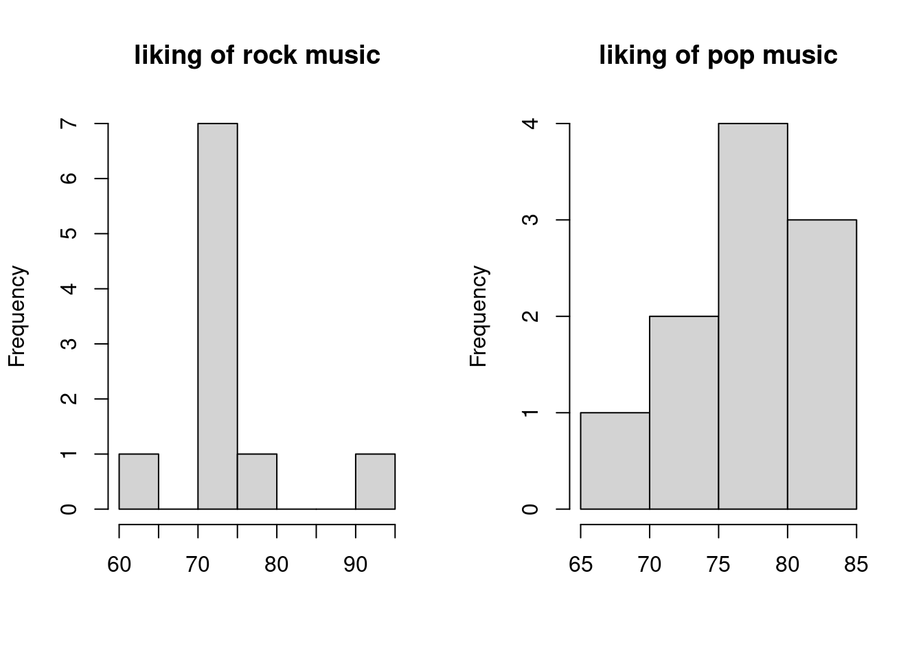 The above histograms show how our simulation with 10 participants would turn out.
As we would expect, with 10 participants the histograms for each group look quite wacky.
The above histograms show how our simulation with 10 participants would turn out.
As we would expect, with 10 participants the histograms for each group look quite wacky.
Previously, we analyzed these data with a paired t-test, for example:
t.test(bivnorm$rock, bivnorm$pop, paired = T)##
## Paired t-test
##
## data: bivnorm$rock and bivnorm$pop
## t = -0.73577, df = 9, p-value = 0.4806
## alternative hypothesis: true difference in means is not equal to 0
## 95 percent confidence interval:
## -9.618983 4.897481
## sample estimates:
## mean of the differences
## -2.360751showing us that there is no difference between the groups, just as we would expect. We could of course also model the same data in a mixed-effects model (we have seen in part II and III of this tutorial how t-tests can be rewritten as linear models).
So lets try this, here comes our first mixed model simulation! However, let us first increase the sample-size to very high so I can demonstrate some important things that we do not want to get distorted by sampling variation in a small sample-size by now. So instead of 10 people let us simulate the same data but with 10,000 people.
data1 <- generate_design(10000, 2, 1)

group_means <- c(rock = 75,pop = 75) # define means of both genres in a vector
rock_sd <- 7.5 # define sd of rock music
pop_sd <- 7.5 # define sd of pop music
correlation <- 0.2 # define their correlation

sigma <- matrix(c(rock_sd^2, rock_sd*pop_sd*correlation, rock_sd*pop_sd*correlation, pop_sd^2), ncol = 2) # define variance-covariance matrix

set.seed(123)
bivnorm <- data.frame(mvrnorm(nrow(data1)/2, group_means, sigma)) # simulate bivariate normal (we use nrow(data1)/2, the number of rows from the data-set above to simulate 10 observations per group)
par(mfrow=c(1,2))
hist(bivnorm$rock, main = "liking of rock music", xlab = "")
hist(bivnorm$pop, main = "liking of pop music", xlab = "")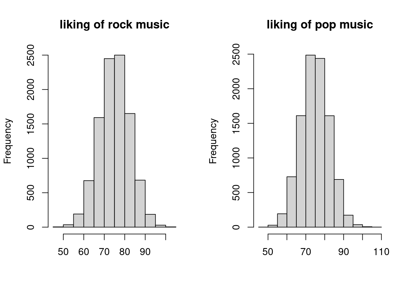
We can already see that the histograms look much more normal now. So let us redo the t-test.
t.test(bivnorm$rock, bivnorm$pop, paired = T) ##
## Paired t-test
##
## data: bivnorm$rock and bivnorm$pop
## t = 0.90922, df = 9999, p-value = 0.3633
## alternative hypothesis: true difference in means is not equal to 0
## 95 percent confidence interval:
## -0.09986109 0.27264389
## sample estimates:
## mean of the differences
## 0.0863914We can immediately see that the difference between groups got smaller, and the confidence interval is more narrow, showing us that we have a much more accurate simulation now.
So now to the mixed model.
First we have to restructure the above data as lme4::lmer uses long-format data, while the bivnorm data that we have has columns for the observations.
bivnorm_dat <- data.frame(cbind(liking = c(bivnorm$rock, bivnorm$pop), genre = c(rep("rock", (nrow(data1)/2)), rep("pop", (nrow(data1)/2))), participant = rep(1:(nrow(data1)/2), 2))) # this just converts bivnorm to long format and adds the genre variable
bivnorm_dat$liking <- as.numeric(bivnorm_dat$liking) # variable was converted to character for some reason in cbind so lets make it numerical again
bivnorm_dat$genre_f <- factor(bivnorm_dat$genre) # make genre a factor

lmer_bivnorm <- lmer(liking ~ genre_f + (1 | participant), bivnorm_dat)
summary(lmer_bivnorm)
## Linear mixed model fit by REML. t-tests use Satterthwaite's method [
## lmerModLmerTest]
## Formula: liking ~ genre_f + (1 | participant)
## Data: bivnorm_dat
##
## REML criterion at convergence: 136955.6
##
## Scaled residuals:
## Min 1Q Median 3Q Max
## -3.3987 -0.6185 0.0035 0.6294 3.8687
##
## Random effects:
## Groups Name Variance Std.Dev.
## participant (Intercept) 11.09 3.330
## Residual 45.14 6.719
## Number of obs: 20000, groups: participant, 10000
##
## Fixed effects:
## Estimate Std. Error df t value Pr(>|t|)
## (Intercept) 74.98622 0.05802 9999.00005 1292.519 <2e-16 ***
## genre_f1 -0.04320 0.04751 9999.00002 -0.909 0.363
## ---
## Signif. codes: 0 '***' 0.001 '**' 0.01 '*' 0.05 '.' 0.1 ' ' 1
##
## Correlation of Fixed Effects:
## (Intr)
## genre_f1 0.000I hope that, in general, you understand the above output, as I assume you are familiar with lme4.
However, let us inspect a few things here:
- The first thing that we might notice is that the Estimate for the effect does actually look smaller than the one from the t-test. This is due to something that we discussed in part III: In the mixed model we use sum-to-zero coding, which shows each group’s deviation from the grand mean (i.e. the mean of pop and rock), which is with two groups, by definition half the total difference between the groups, which is what the t-test shows. We can verify that indeed double the estimate of the mixed model,
-0.04320*2 =-0.0864, which is very close to the0.0863914of the t-test estimate of the group difference. The fact that in one case the estimate is positive, and in the other it is negative, is just because a different reference level is used. If you switch the order of groups in the t-test above, the estimate will get negative as well. - Compared to the t-test, we also get an estimate for the intercept, representing the grand mean, just as we do in normal linear models. This is very close to the 75 mean that we simulated.
- The degrees of freedom are close to the ones from the t-test, BUT, they are a little weird in that they are decimal numbers. Unless you have used mixed models a lot, this might seem odd. However, there are reasons for this (that I do not want to go into too much), but you can see this as an indicator that we get into a complicated domain where the mixed model is not exactly comparable to the t-test, or a repeated-measures ANOVA approach to this data. However, that should not bother us too much at the moment - it suffices to realize that the df is similar to the one from the t-test, i.e. 9999 (
participants per group - 1) in this case.
One thing that might appear odd however, is that, if you look at the output of the mixed-model, we cannot find our simulated standard deviations of 7.5.
Did something go wrong? And where should we find them anyway? Should they be found as the residual variance? Or the participant random effect variance? Or should they be in the standard error of the effect? And where is our correlation of .20?
Let us investigate…
Another correlation-based detour
We have dealt with correlations and simulations extensively in part II, and again, the correlations here play a main role in solving this case.
As we are working with mvrnorm in this case, we supplied the function with a variance-covariance matrix (see part II for more explanation) for the variance, sigma <- matrix(c(rock_sd^2, rock_sd*pop_sd*correlation, rock_sd*pop_sd*correlation, pop_sd^2), ncol = 2), a matrix containing the variances of both groups (rock and pop) and their covariance that looks like this:
As both groups have the same variance there are only 2 different numbers in the matrix, namely the variance of each group, i.e. rock_sd^2 = 56.25 and pop_sd^2 = 56.25 and the covariances between the groups rock_sd*pop_sd*correlation = 11.25 (note that the covariances would be the same even if the group variances were not the same in both groups, as by definition, 2 groups can only have one covariance, i.e. the same formula is used twice in the matrix).
Thus, these two numbers should somewhere to be found in the model output, or not?
Indeed, they are and to find these numbers in the model output, we have to understand what they mean.
Let us have a look at the random effects terms, that capture the variance in components in mixed models:
Participant random variance
The Participant variance in the random effects terms of the model is the variance that we can attribute to participants, in this case it is 11.09.
That this variance is greater than 0 tells us that some variance in liking ratings of pop and rock music can be attributed to participants.
In other words, knowing a participant’s rating of pop music, we will carry some information about a participant’s rating of rock music.
This, as you might realize, sounds suspiciously like a correlation between the liking ratings across participants, and, just as suspiciously 11.09 is very close to the simulated covariance of 11.25 above.
So, might this number represent the correlation between the ratings?
As covariances are just a unstandardized correlation, we can actually check this.
For instance, if from he covariance of 11.25 from the simulation, we want to go back to the underlying correlation, we divide it by the product of the group SDs rock_sd*pop_sd, i.e. 11.25/(7.5*7.5) = 0.2, the specified correlation from above.
In the simulated data, the correlation that we actually observed was 0.1971886 and indeed (if we use the unrounded value of the participant SD that we get with VarCorr(lmer_bivnorm)[[1]][1]) we find: 11.08745/(sd(subset(bivnorm_dat, genre == "rock")$liking)*sd(subset(bivnorm_dat, genre == "pop")$liking))) = 0.1971886.
First riddle solved, the participant random variance is indeed the specified covariance!
Residual random variance
What about the Residual variance in the model output? Why does it not correspond to the other variance component in the matrix above, namely 56.25.
The residual represents the variance that cannot be attributed to any sources that we understand, i.e. sources that we model.
So first of all let us look at how much total variation there is in the data.
The total variance is just the mean variance of all scores in the two groups var(subset(bivnorm_dat, genre == "rock")$liking)+var(subset(bivnorm_dat, genre == "pop")$liking)/2 = 56.2286228.
As mentioned, he residual variance is the part of this variance that we do not know what it can be attributed to.
However, just a minute ago, we already attributed some of the variance to the participants - so we can deduct this variance, as it is not part of the residual anymore:
(var(subset(bivnorm_dat, genre == "rock")$liking)+var(subset(bivnorm_dat, genre == "pop")$liking))/2-11.08745 = 45.14 which is again, exactly what we see in the model.
Some important Remarks on this variance decomposition
It is important to mention a few things here. As you might have realized by now, finding the simulated variances in the model output is not always trivial. When models get more complex, various variances might influence different terms, and in mixed models designs, we often might deal with unbalanced data, where the group sizes are not always equal. Thus, do not expect this method to generalize to more complex designs - this was mainly a demonstration to show that mixed models are not totally “crazy” and give us weird numbers but that the numbers do indeed bear some relation to the more “simple” statistical models we worked with before. However, this meaning might sometimes be more difficult to trace. After all, this is not even a bad thing - we use mixed models to model things that are complicated, and we want the model to figure out what to do with e.g. unbalanced designs etc. If we would just be able to do the same thing with calculating some variances by hand, we would not need a mixed model after all.
An easy way to “break” mixed models
Consider a slightly different assumption about the correlation between liking scores. It is very much possible that a participant who likes rock music will dislike pop music. Thus, knowing a rock music score for a certain participant, we could expect the next score to be somewhat lower and vice versa, i.e. there would be negative correlation between the scores. If we change the above correlation in the simulation to be negative, we will get a rather weird output for the mixed model however:
correlation_neg <- -0.2 # now correlation is negative

sigma_neg <- matrix(c(rock_sd^2, rock_sd*pop_sd*correlation_neg, rock_sd*pop_sd*correlation_neg, pop_sd^2), ncol = 2) # define variance-covariance matrix

set.seed(123)
bivnorm_neg <- data.frame(mvrnorm(nrow(data1)/2, group_means, sigma_neg))

bivnorm_dat_neg <- data.frame(cbind(liking = c(bivnorm_neg$rock, bivnorm_neg$pop), genre = c(rep("rock", (nrow(data1)/2)), rep("pop", (nrow(data1)/2))), participant = rep(1:(nrow(data1)/2), 2)))
bivnorm_dat_neg$liking <- as.numeric(bivnorm_dat_neg$liking)
bivnorm_dat_neg$genre_f <- factor(bivnorm_dat_neg$genre)

lmer_bivnorm_neg <- lmer(liking ~ genre_f + (1 | participant), bivnorm_dat_neg)
## boundary (singular) fit: see ?isSingularsummary(lmer_bivnorm_neg)## Linear mixed model fit by REML. t-tests use Satterthwaite's method [
## lmerModLmerTest]
## Formula: liking ~ genre_f + (1 | participant)
## Data: bivnorm_dat_neg
##
## REML criterion at convergence: 137352.1
##
## Scaled residuals:
## Min 1Q Median 3Q Max
## -4.0155 -0.6738 0.0063 0.6787 3.5617
##
## Random effects:
## Groups Name Variance Std.Dev.
## participant (Intercept) 0.00 0.000
## Residual 56.23 7.499
## Number of obs: 20000, groups: participant, 10000
##
## Fixed effects:
## Estimate Std. Error df t value Pr(>|t|)
## (Intercept) 75.04320 0.05302 19998.00000 1415.30 <2e-16 ***
## genre_f1 -0.01378 0.05302 19998.00000 -0.26 0.795
## ---
## Signif. codes: 0 '***' 0.001 '**' 0.01 '*' 0.05 '.' 0.1 ' ' 1
##
## Correlation of Fixed Effects:
## (Intr)
## genre_f1 0.000
## optimizer (nloptwrap) convergence code: 0 (OK)
## boundary (singular) fit: see ?isSingularFirst we get a warning about the fit being “singular”. Second, we see that, even though the absolute covariance is just as large this time but negative (-11.25), the model tells us that the covariance of participants is 0!! Can that be right? The correlation is indeed -0.1971886 so using the formula to infer the covariance from the group SDs in the data we would expect
cor(subset(bivnorm_dat_neg, genre == "rock")$liking, subset(bivnorm_dat_neg, genre == "pop")$liking)
*sd(subset(bivnorm_dat_neg, genre == "rock")$liking)
*sd(subset(bivnorm_dat_neg, genre == "pop")$liking)
== 0
It is, however, -11.0874483, which is certainly not 0! However, take a moment to reflect on how a variance is defined as the squared standard-deviation, i.e. \(var = sd^2\). By definition, a squared number cannot be negative, and therefore the variance can also never be negative. Mixed models have a built-in restriction that honors this notion. If a covariance is negative, the mixed model gives us the closest number that it assumes reasonable for a random effect variance, namely 0 which is just an SD of 0 squared, and will tell us that the model is “singular” i.e. the variance component cannot be estimated.
Anova procedures do not “suffer” from this problem, as they use a sum-of-squares approach, where the sum-of-squares are always positive. This means that in cases where the observed correlation between the observations is negative, Anovas and mixed models will yield different results:
ez_an <- ez::ezANOVA(bivnorm_dat_neg, dv = .(liking), wid = .(participant), within = .(genre_f), detailed = T)

print(ez_an)
## $ANOVA
## Effect DFn DFd SSn SSd F p
## 1 (Intercept) 1 9999 112629624.416931 451366.6 2495053.03358603 0.0000000
## 2 genre_f 1 9999 3.796855 673093.4 0.05640339 0.8122785
## p<.05 ges
## 1 * 0.990114992309
## 2 0.000003376591Which one is the true result though? Both and neither, it is just a design choice that package developers made. As Jake Westfall put it better than I ever could for models that have these negative covariances:
“The best-fitting model is one that implies that several of the random variance components are negative. But lmer() (and most other mixed model programs) constrains the estimates of variance components to be non-negative. This is generally considered a sensible constraint, since variances can of course never truly be negative. However, a consequence of this constraint is that mixed models are unable to accurately represent datasets that feature negative intraclass correlations, that is, datasets where observations from the same cluster are less (rather than more) similar on average than observations drawn randomly from the dataset, and consequently where within-cluster variance substantially exceeds between-cluster variance. Such datasets are perfectly reasonable datasets that one will occasionally come across in the real world (or accidentally simulate!), but they cannot be sensibly described by a variance-components model, because they imply negative variance components. They can however be”non-sensibly" described by such models, if the software will allow it. aov() allows it. lmer() does not".
A second, very important point to mention is that lme4 actually scales the random effect terms by the residual variance when estimating them.
What this means is that, as far as the fitting algorithm is concerned, a model with a random intercept SD of 10 and a residual SD of 20 is exactly identical to a model where the random intercept SD would be 100 and the residual would be 200 or a model where the random intercept SD would be 1 and the residual SD would be 2, at least regarding the random effect structures.
All that the model cares about is that the random intercept is 0.5 times the residual SD.
What this means for us is that when specifying the random effect structure, we do not actually need to keep the scale of the response in mind if that is difficult to do.
In my experience, in my own research where I work a lot with rating scales and/or binary decisions, keeping estimates on the original scale often helps me figuring out what effect sizes I expect but I can imagine that there are many situations in which this is not so easy.
Thus, it is good to know that in those situations you can just think about the residual SD first and then derive how much smaller / bigger you expect the random effects to be relative to the residual.
Back on track: Simulating a DV based on the data-frame row entries
I hope you forgive this rather long detour, but I felt that it was important to clarify how simulations for mixed models relate to simulations for simpler models. In the beginning of this tutorial, I mentioned that we would now use a simulation approach in which we would calculate each value for the DV directly from the other values in the data-frame for each row (i.e. directly from the design matrix). As we want to build more complicated models now, we have to leave the direct group mean simulation approach from before behind and move on to the regression weight simulation approach that I will now describe. It involves writing up the simulation in terms of a linear model notation once more (see part II and part III of this tutorial). This is not entirely new as we used linear models to simulate ANOVA designs before in part III, but what is new is that now we are not simulating groups directly before and use dummy variables for each factor but rather use a pre-baked dataset that entails all information for us to calculate the DV for each row of the dataset.
If we write the above model down in a linear model notation we get:
\[ y_i = \beta_0 + \beta_1genre_i + \epsilon_i \]
In the regression weight simulation approach, we will still start of with thinking about the (group) means. However, we will simulate each observation of the dependent variable \(y_i\) by directly using a regression equation describing the regression model that produces our expected means. Thus, for each row, the value for \(y_i\) (i.e. the liking of the particular song for the particular genre for a particular participant) will be the sum specified above.
The problem that we need to solve is that we need to figure out what \(beta_0\) and \(beta_1\) are to be able to calculate \(y_i\).
In this model, \(\beta_0\) represents the grand mean (mean of all expected group means), which is \(\mu_{grand} = (\mu_{rock}+\mu_{pop})/2 \Rightarrow \mu_{grand} = (75+75)/2 \Rightarrow \beta_0 = 75\)
As we use sum-to-zero coding for factors again (see part III of the tutorial), \(\beta_1\) represents the deviation from \(beta_0\) depending on the respective group.
We start by making genre a factor variable.
data1$genre_f <- factor(data1$genre) # make a new variable for the factor
contrasts(data1$genre_f)
## [,1]
## pop 1
## rock -1We see that when genre_f in the data is equal rock, it will assume the value -1 in our linear model, while it will assume the value 1 for pop.
If we put this information in the model we can calculate the \(beta_1\) by filling in one of the group means, for instance \(\mu_{rock}\):
For instance, we can calculate \(\mu_{rock} = \beta_0 + \beta_1*genre_i\)
We specified that \(\mu_{rock} = 75\), and we just calculated that \(\beta_0 = 75\).
Moreover, we know that \(genre_i\) in this case is rock, so in the regression equation it will become -1:
\(75 = 75 + \beta_1*-1\). Solving this equation to \(beta_1\) yields \(0 =\beta_1*-1 \Rightarrow \beta_1 = 0\). This is unsurprisingly representing our initial wish that there should be no difference between group means.
The remaining part of the equation, \(\epsilon\), is the error that we specified above as sigma in mvrnorm.
If we write this down in simulation code we get:
data1$genre_pop <- ifelse(data1$genre == "pop", 1, -1)
b0 <- 75
b1 <- 0
epsilon <- 7.5
set.seed(1)
for(i in 1:nrow(data1)){
  data1$liking[i] <- rnorm(1, b0+b1*data1$genre_pop[i], epsilon)
  # we simulate a normal distribution here with the mean being the regression equation (except the error term) and the SD being the error term of the regression equation
}

lmem1 <- mixed(liking ~ genre + (1 | participant), data1, method = "S")
## Fitting one lmer() model. [DONE]
## Calculating p-values. [DONE]summary(lmem1)## Linear mixed model fit by REML. t-tests use Satterthwaite's method [
## lmerModLmerTest]
## Formula: liking ~ genre + (1 | participant)
## Data: data
##
## REML criterion at convergence: 137424.4
##
## Scaled residuals:
## Min 1Q Median 3Q Max
## -4.2766 -0.6696 -0.0125 0.6715 3.7953
##
## Random effects:
## Groups Name Variance Std.Dev.
## participant (Intercept) 0.2734 0.5228
## Residual 56.1596 7.4940
## Number of obs: 20000, groups: participant, 10000
##
## Fixed effects:
## Estimate Std. Error df t value Pr(>|t|)
## (Intercept) 74.959773 0.053248 9998.985098 1407.756 <2e-16 ***
## genre1 0.008801 0.052990 9998.984622 0.166 0.868
## ---
## Signif. codes: 0 '***' 0.001 '**' 0.01 '*' 0.05 '.' 0.1 ' ' 1
##
## Correlation of Fixed Effects:
## (Intr)
## genre1 0.000You can see that in the above for-loop we do nothing but simulate, from a normal distribution, one observation for each row of the data-set where the specific genre in that row is taken into account.
The mean of the normal distribution for each row is the regression equation defined above, excluding \(\epsilon\), transferred into R-code.
\(\epsilon\) enters the model as the SD of this normal distribution, thereby taking its role as the error term.
All values are just as we would expect. We did not define any random intercept variance in the simulation code above, therefore we do only get very small (simulation variance) values and get a value close to 7.5 for \(\epsilon\).
Building up the random effects structure
Adding a random intercept
However, usually, the reason why we would use mixed models is because we think that there will be covariance. So how do we put our expectation that people who like music more in general will like either genre more into the model using the regression weight simulation approach? We do this by adding another term into the regression equation, that tracks a special value for each participant representing their “general liking of music”. More specifically, it tracks the difference from a specific participant from the mean music liking - their random intercept:
\[ y_{ij} = \beta_0 + u_{0j} + \beta_1genre_{i} + \epsilon_{i} \] As you can see in the equation above, we got a new index \(_j\) for the terms that were in the model previously (by the way beta_0 has no index as it the same for each row and does not depend on other variables). This index tracks the participant number in each row. Thus if \(_j = 1\) we are looking at values of participant 1 - either their liking of rock or pop music. This index is important for the new term \(u\) in the model, that represents the random intercept of the participant, which is their average deviation from the average music liking in the sample. In other words if \(u0_1 = 10\) it means that the average liking of participant 1 for pop and rock music is 10 points higher than the average liking in the sample. As it also represents an intercept (just as \(\beta_0\)) we also add the 0 here in the notation.
If we want to put our correlation of .20 in the simulation again, we can do so via calculating the random SD values that these would represent again (i.e. \(\sqrt{11.25}\) for the random intercept and and \(\sqrt{56.25-11.25}\) for the residual). Next, we can put a new term in the simulation that generates \(J\) different values for \(u0_j\) representing one intercept value for each participant that is applied based on the participant number in each row of our data-set.
b0 <- 75
b1 <- 0
sd_u0 <- sqrt(11.25)
epsilon <- sqrt(56.25-11.25)
U0 = rnorm(length(unique(data1$participant)), 0, sd_u0)
str(U0)
## num [1:10000] 0.789 0.821 -2.154 -6.49 3.484 ...This is how we would simulate the random intercept values. We specify the SD of the random intercept values \(sd_{uj}\) and use it to sample from a distribution with mean 0 (the mean of random intercepts is always 0 by definition as they represent a deviation from the mean which, logically, must have a mean of 0) and a standard-deviation of \(sd_{uj}\). We sample 10,000 values from this distribution, 1 for each participant. Next we need to put this into the mean simulation.
set.seed(1)
for(i in 1:nrow(data1)){
  data1$liking[i] <- rnorm(1, b0+U0[data1$participant[i]]+b1*data1$genre_pop[i], epsilon)

}

lmem2 <- mixed(liking ~ genre + (1 | participant), data1, method = "S")
## Fitting one lmer() model. [DONE]
## Calculating p-values. [DONE]summary(lmem2)## Linear mixed model fit by REML. t-tests use Satterthwaite's method [
## lmerModLmerTest]
## Formula: liking ~ genre + (1 | participant)
## Data: data
##
## REML criterion at convergence: 137041.6
##
## Scaled residuals:
## Min 1Q Median 3Q Max
## -3.5076 -0.6185 -0.0083 0.6163 3.5313
##
## Random effects:
## Groups Name Variance Std.Dev.
## participant (Intercept) 11.65 3.413
## Residual 44.93 6.703
## Number of obs: 20000, groups: participant, 10000
##
## Fixed effects:
## Estimate Std. Error df t value Pr(>|t|)
## (Intercept) 74.989359 0.058404 9998.999983 1283.978 <2e-16 ***
## genre1 0.007872 0.047396 9998.999952 0.166 0.868
## ---
## Signif. codes: 0 '***' 0.001 '**' 0.01 '*' 0.05 '.' 0.1 ' ' 1
##
## Correlation of Fixed Effects:
## (Intr)
## genre1 0.000As you can see from the output, we get exactly what we would expect.
Note that it was very easy to add the random intercept to the model, we just added the term U[data1$participant[i]] to the existing 1-liner for the simulation.
If you are unfamiliar with indexing in R, this does nothing more than say that for each row i we want the value from the random intercept list U that belongs to the participant that we see at row i.
To make the random intercept simulation more traceable we can plot it. If we use the code above, but set the error term \(\epsilon\) to a very small number, we will see what influence the random effect has on the data.
epsilon_noerror <- .001
data1_noerror <- subset(data1, participant <= 20) # take only 20 participants for plotting
set.seed(1)
for(i in 1:nrow(data1_noerror)){
data1_noerror$liking[i] <- rnorm(1, b0+U0[data1_noerror$participant[i]]+b1*data1_noerror$genre_pop[i], epsilon_noerror)
}
ggplot(data1_noerror, aes(x=genre, y=liking, colour=factor(participant), group = factor(participant))) + geom_line()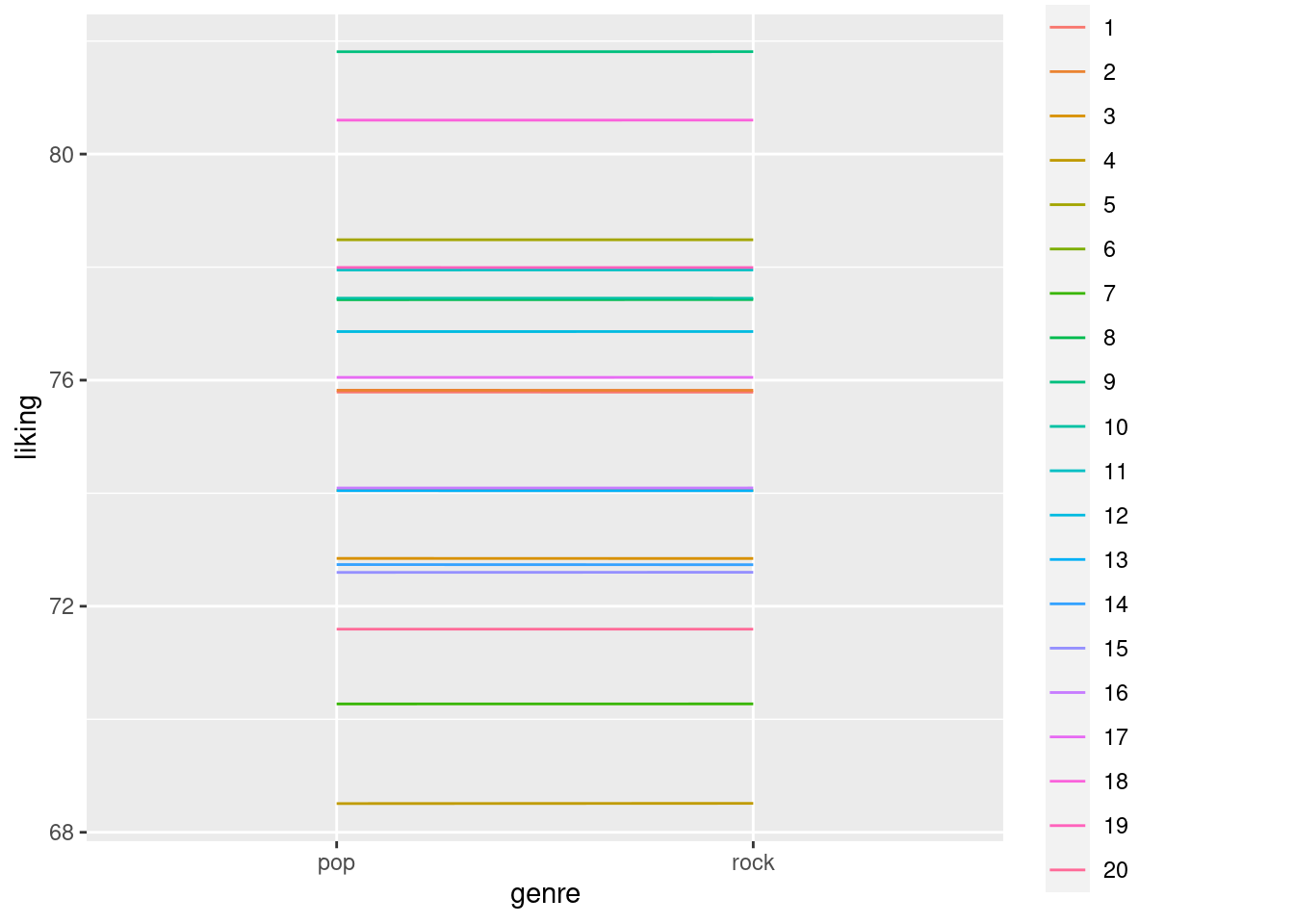 We can see in the above plot that each participant has exactly no difference in liking for rock and pop music, as \(beta_1\) is 0 and there is no error term that causes random variations.
Still, the likings of each participant differ, as the random intercept causes overall ratings to be lower or higher for different participants.
We can see in the above plot that each participant has exactly no difference in liking for rock and pop music, as \(beta_1\) is 0 and there is no error term that causes random variations.
Still, the likings of each participant differ, as the random intercept causes overall ratings to be lower or higher for different participants.
Adding a random slope
Now, we might have the (reasonable) expectation that, while on average, the difference in liking between the two genres is 0 (represented by our fixed effect \(beta_1\) being 0), different people might still prefer one genre over the other, but that variation is just random in that we do not know where it comes from. Still, it might be there and we might want to model it using a random slope for the genre across participant, tracking, for each participant, what their personal difference from the average genre effect i.e. 0 is. In other word, we now expect that it is rarely the case that each participant likes rock and pop exactly the same. Rather, each participant has a preference but these preferences average out across the sample to be 0. We can add this to the regression equation again:
\[ y_{ij} = \beta_0 + u_{0j} + (\beta_1+u_{1j})\times genre_{i} + \epsilon_{i} \]
this equation denotes the fact the value for genre (1 or -1 representing rock and pop) does not only depend on \(beta_1\) but also the random slope term \(u_{1j}\). As you can see above the terms \(beta_1\) and \(u_{1j}\) are between brackets, so they need to be figured out before multiplying them with the value for genre. However, with the current design, we cannot attempt such a stunt, as each participant provides only 2 ratings (1 song from each genre).
Thus, only 1 possible difference score can be calculated per participant. From this single difference score, it is of course not possible to estimate two distinct parameters, namely the average effect \(beta_0\) across participants as well as the average deviation of each participant from that effect. We can only do this if each participant rates more than 2 songs per genre so that two quantities can be distinguished in the model.
Thus, we will now change our data-set a little, so that each participant provides ratings of not only 1 but 20 songs.
We already did this in data2 in the beginning of this tutorial and will now just add more participants to that data:
data2 <- generate_design(n_participants = 500, n_genres = 2, n_songs = 20) # note that we pass the number of songs per GENRE
str(data2)
## 'data.frame': 20000 obs. of 3 variables:
## $ participant: int 1 2 3 4 5 6 7 8 9 10 ...
## $ genre : chr "rock" "rock" "rock" "rock" ...
## $ song : chr "rock_1" "rock_1" "rock_1" "rock_1" ...
## - attr(*, "out.attrs")=List of 2
## ..$ dim : Named int [1:3] 500 2 20
## .. ..- attr(*, "names")= chr [1:3] "participant" "genre" "song"
## ..$ dimnames:List of 3
## .. ..$ participant: chr [1:500] "participant= 1" "participant= 2" "participant= 3" "participant= 4" ...
## .. ..$ genre : chr [1:2] "genre=1" "genre=2"
## .. ..$ song : chr [1:20] "song= 1" "song= 2" "song= 3" "song= 4" ...We have 500 participants now in data2, so that the overall number of observations is the same as in data1 for now.
Now, how big do we think that the random slope should be? The number should represent our expectation about the range that any given person’s difference in liking between rock and pop music should be in. For instance, if we take the normal distribution quantities and use a 2-SD rule, we could think that 95% of people should not have a difference in the 2 likings stronger than 10 points. If we divide that by 2, we get 5 as an sd for the random slope.
data2$genre_pop <- ifelse(data2$genre == "pop", 1, -1)
b0 <- 75
b1 <- 0
sd_u0 <- sqrt(11.25)
epsilon <- sqrt(56.25-11.25)
U0 = rnorm(length(unique(data2$participant)), 0, sd_u0)

sd_u1 = 5
U1 = rnorm(length(unique(data2$participant)), 0, sd_u1)
str(U1)
## num [1:500] -2.092 1.776 2.567 0.093 6.592 ...The above code shows that, again, we get 1 score per participant for the random intercept and random slope.
set.seed(1)
for(i in 1:nrow(data2)){
  data2$liking[i] <- rnorm(1,
                           b0+U0[data2$participant[i]]+
                           (b1+U1[data2$participant[i]])*data2$genre_pop[i],
                           epsilon)

}

lmem3 <- mixed(liking ~ genre + (1 + genre | participant), data2, method = "S", control = lmerControl(optimizer = "bobyqa"))
## Fitting one lmer() model. [DONE]
## Calculating p-values. [DONE]summary(lmem3)## Linear mixed model fit by REML. t-tests use Satterthwaite's method [
## lmerModLmerTest]
## Formula: liking ~ genre + (1 + genre | participant)
## Data: data
## Control: lmerControl(optimizer = "bobyqa")
##
## REML criterion at convergence: 135817.2
##
## Scaled residuals:
## Min 1Q Median 3Q Max
## -3.8360 -0.6544 -0.0134 0.6536 3.5644
##
## Random effects:
## Groups Name Variance Std.Dev. Corr
## participant (Intercept) 11.42 3.379
## genre1 28.33 5.323 -0.03
## Residual 45.21 6.724
## Number of obs: 20000, groups: participant, 500
##
## Fixed effects:
## Estimate Std. Error df t value Pr(>|t|)
## (Intercept) 74.9965 0.1584 499.0000 473.407 <2e-16 ***
## genre1 -0.2564 0.2427 498.9999 -1.056 0.291
## ---
## Signif. codes: 0 '***' 0.001 '**' 0.01 '*' 0.05 '.' 0.1 ' ' 1
##
## Correlation of Fixed Effects:
## (Intr)
## genre1 -0.025Unsurprisingly, the output above shows the amount of random slope variance that we intended to simulate.
Again we can plot this combination of random slope + intercept.
data2_noerror <- subset(data2, participant <= 20) # take only 20 participants for plotting
set.seed(1)
for(i in 1:nrow(data2_noerror)){
data2_noerror$liking[i] <- rnorm(1,
b0+U0[data2_noerror$participant[i]]+
(b1+U1[data2_noerror$participant[i]])*data2_noerror$genre_pop[i],
epsilon_noerror)
}
ggplot(data2_noerror, aes(x=genre, y=liking, colour=factor(participant), group = factor(participant))) + geom_line()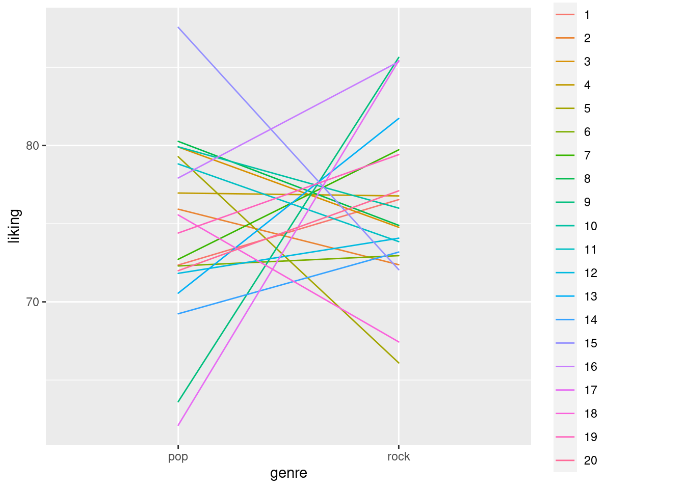 We can now see that not only does each participant still have a different mean, they also have do not have flat slopes anymore, but can have even large differences in their liking for pop vs. rock music.
However, across all participants the difference is still zero.
We can now see that not only does each participant still have a different mean, they also have do not have flat slopes anymore, but can have even large differences in their liking for pop vs. rock music.
However, across all participants the difference is still zero.
Adding random term correlations
We can see that in the above model output, we get a small number next to the random slope. This number -0.03 is the correlation between the random terms. It means that if the random intercept for a specific participant is high, the slope would also be highly positive and vice versa. In our situation, this correlation can be helpful in addressing the problem that in order to have a really high random intercept, you should have very high likings for both genres. For instance, a person can only have an average liking of 100, if they have a liking of 100 for both, rock and pop. Thus, we can expect a negative correlation between the random intercept and slope, where high liking (high random intercepts) is related to lower differences in liking (lower random slopes).
Luckily, we do not have to use any new tricks here, we can just make use of the mvrnorm function again, but this time, instead of using it to simulate correlated groups, we will use it for the simulation of the random terms \(u_{0j}\) and \(u_{1j}\).
We could, for instance assume a negative correlation of -.20
set.seed(1)
b0 <- 75
b1 <- 0
sd_u0 <- sqrt(11.25)
epsilon <- sqrt(56.25-11.25)
sd_u1 <- 5
corr_u01 <- -.20
sigma_u01 <- matrix(c(sd_u0^2, sd_u0*sd_u1*corr_u01, sd_u0*sd_u1*corr_u01, sd_u1^2), ncol = 2)

U01 <- mvrnorm(length(unique(data2$participant)),c(0,0),sigma_u01)
str(U01)
## num [1:500, 1:2] 0.472 0.726 4.686 -1.858 -3.504 ...
## - attr(*, "dimnames")=List of 2
## ..$ : NULL
## ..$ : NULLcor(U01)[2]## [1] -0.1446309We can see that we got a matrix with 2 rows of 500 observations each and that their correlation is cor(U01)[2] = -0.1446309, which is not exactly what we wanted, but relatively close.
The difference is due to the fact that for the correlation, there are only 500 pairs of scores that can be used to estimate it and it is therefore relatively unstable (try increasing the size of U01 to 10,000 observations for example and you will see that it is much closer to what we would expect).
Now, we have to put this into the model again.
for(i in 1:nrow(data2)){
  data2$liking[i] <- rnorm(1,
                           b0+U01[data2$participant[i], 1]+
                           (b1+U01[data2$participant[i], 2])*data2$genre_pop[i],
                           epsilon)

}

lmem4 <- mixed(liking ~ genre + (1 + genre | participant), data2, method = "S", control = lmerControl(optimizer = "bobyqa"))
## Fitting one lmer() model. [DONE]
## Calculating p-values. [DONE]summary(lmem4)## Linear mixed model fit by REML. t-tests use Satterthwaite's method [
## lmerModLmerTest]
## Formula: liking ~ genre + (1 + genre | participant)
## Data: data
## Control: lmerControl(optimizer = "bobyqa")
##
## REML criterion at convergence: 135757.9
##
## Scaled residuals:
## Min 1Q Median 3Q Max
## -3.9311 -0.6568 -0.0113 0.6562 3.6397
##
## Random effects:
## Groups Name Variance Std.Dev. Corr
## participant (Intercept) 12.18 3.489
## genre1 25.71 5.070 -0.16
## Residual 45.13 6.718
## Number of obs: 20000, groups: participant, 500
##
## Fixed effects:
## Estimate Std. Error df t value Pr(>|t|)
## (Intercept) 75.1087 0.1631 499.0003 460.45 <2e-16 ***
## genre1 0.1299 0.2317 498.9998 0.56 0.575
## ---
## Signif. codes: 0 '***' 0.001 '**' 0.01 '*' 0.05 '.' 0.1 ' ' 1
##
## Correlation of Fixed Effects:
## (Intr)
## genre1 -0.153As you can see, the only thing that changed here is that we are using the matrix of random intercept and slope values here for the simulation here by assessing it at column 1 (U01[data2$participant[i], 1]) for the random intercepts and column 2 (U01[data2$participant[i], 2]) for the random slopes.
Adding a crossed random effects term.
It is possible, that some songs are universally more liked across people than others.
For example if we imagine for a moment that the song pop_1 in our data-set represents, for example Blank Space by Taylor Swift - obviously an amazing song that most people will like.
Similarly, universally liked songs might be in the rock genre and also similarly, there might be songs in both genres that most people do not like so much (remember though that we are working with a “most liked” playlist from Spotify so it makes sense that regardless our overall mean of 75 stays the same).
Thus, it is not only the fact that people differ in their general liking of music, but also that songs differ in their propensity to be liked. To represent this we can add another random intercept representing songs:
\[ y_{ijk} = \beta_0 + u_{0j} + w_{0k} + (\beta_1+u_{1j})\times genre_{i} + \epsilon_{i} \] The new term \(w_{0k}\) is doing just what I described above, and is very similar to \(u_{0j}\) but it represents the term \(w\), a term that tracks the deviation from the overall liking scores for each given song \(_k\).
We can, for instance, assume that the random intercept for songs will be half the size of random intercepts across people, making the assumption that differences between people are often larger than differences between things, in this case songs.
sd_w0 <- sqrt(11.25)/2
W0 <- rnorm(length(unique(data2$song)), 0, sd_w0) # note how we use the number of songs here to specify the size of W0 instead of the participant number
We can now just add this to the simulation of the DV again and add the random intercept to the lmer syntax.
Note that in the code below, we need a way to index to the right song for each value in W0.
For participants this was easy, as participant numbers are just numerals from 1-J that automatically also represent index values.
For songs however, the syntax data2$song[i] will not return a number, but, for instance rock_1, as this is the song ID.
We could either covert song IDs to numbers as well, or we can use syntax that retrieves the index of, for example rock_1 in the list of unique songs.
This is what the slightly confusing W0[which(unique_songs == data2$song[i])] syntax does.
Note that we create unique_songs outside of the loop, because creating the list of unique songs causes R to do a search across the entire data-set for unique song names, and it suffices to do this once instead of every iteration of the loop.
You will note that the code will run significantly slower if you put it inside of the loop.
unique_songs <- unique(data2$song)
for(i in 1:nrow(data2)){
  data2$liking[i] <- rnorm(1,
                           b0+U01[data2$participant[i], 1] +
                           W0[which(unique_songs == data2$song[i])] +
                           (b1+U01[data2$participant[i], 2])*data2$genre_pop[i],
                           epsilon)

}

lmem5 <- mixed(liking ~ genre + (1 + genre | participant) + (1 | song), data2, method = "S", control = lmerControl(optimizer = "bobyqa"))
## Fitting one lmer() model. [DONE]
## Calculating p-values. [DONE]summary(lmem5)## Linear mixed model fit by REML. t-tests use Satterthwaite's method [
## lmerModLmerTest]
## Formula: liking ~ genre + (1 + genre | participant) + (1 | song)
## Data: data
## Control: lmerControl(optimizer = "bobyqa")
##
## REML criterion at convergence: 135951.7
##
## Scaled residuals:
## Min 1Q Median 3Q Max
## -3.9684 -0.6629 0.0116 0.6474 3.4745
##
## Random effects:
## Groups Name Variance Std.Dev. Corr
## participant (Intercept) 12.47 3.531
## genre1 25.39 5.038 -0.13
## song (Intercept) 5.20 2.280
## Residual 45.21 6.724
## Number of obs: 20000, groups: participant, 500; song, 40
##
## Fixed effects:
## Estimate Std. Error df t value Pr(>|t|)
## (Intercept) 75.0514 0.3965 53.5030 189.291 <2e-16 ***
## genre1 0.3312 0.4278 71.8909 0.774 0.441
## ---
## Signif. codes: 0 '***' 0.001 '**' 0.01 '*' 0.05 '.' 0.1 ' ' 1
##
## Correlation of Fixed Effects:
## (Intr)
## genre1 -0.028We can see that the random intercept SD is slightly higher than we wanted to simulate, but this is not surprising given that there are only 40 different songs that the random intercept SD is simulated over. If we would increase the number of songs to, say 10,000, the value would be much closer to what we expect. However, if we would want to keep the number of participants the same we would also have a data-set of 5,000,000 rows, and it would take ages to estimate, and it is also not a realistic design to have people listen to 10,000 songs each.
Should we add the genre random slope for songs as well? Try to think about this for a second. What would it mean to add the random slope for genre across songs here? It would mean that we would expect a certain song to differ in its propensity to be liked as a pop song compared to being liked as a rock song. Clearly, this does not make sense as a song is either rock or pop but cannot “switch” genre from rock to pop or vice versa. Thus, genre is a within-participant factor here but it is between-songs meaning that we cannot add a random slope here as it does not make sense.
Adding a second-order (nested) random term
It could be possible that the liking that people show for music also depend on what country they live in as music could be more or less important in a culture. To address this, we could add a random term that identifies different countries. For instance, we could assume that our 500 participants in this simulation come from 5 different countries (I am not qualified to make any actual statements about which countries would show which effect and do not want to imply things only for the sake of an example so I will just call the countries Country A - Country E). We can also assume that the countries are of different size so that they will not be equally represented by the 500 people in our sample.
country_list <- sample(c("A", "B", "C", "D", "E"),size = length(unique(data2$participant)), prob = c(0.25, 0.15, 0.05, 0.35, 0.2), replace = T)
table(country_list)
## country_list
## A B C D E
## 133 64 20 173 110Using the sample command, we sampled a list that contains 500 letters from A-E representing countries, one for each participant.
The countries relative size is defined by the prob argument (e.g. country A is assumed to have 5 times the population of country C).
We can now add these countries to the data-frame:
for(i in 1:nrow(data2)){
  data2$country[i] <- country_list[data2$participant[i]]
}
Above, I mentioned that we are working with a nested rather than a crossed effect here. However, for simulation, this does actually not matter much, because, as Robert Long mentions: “Nesting is a property of the data, or rather the experimental design, not the model.” For us, this means that we can add nested random effects just as we can add crossed effects. However, it might make sense (depending on the situation) to make nested effects’ size depend on each other. For instance, we might think of it like this: knowing the country that a person is from already tells us something about their music liking. Having this information does not explain previously unexplained variance, because the variance was already there, but it was attributed to the person not knowing what “caused” it. For instance, we could assume that 10% of the variance that is no attributed to the random intercept of participants can actually be attributed to country.
Thus we could decrease the size of the random terms for participant by 10 percent and move that 10 percent variance to the random term for country.
The country random term CU01 will then look like this:
sd_cu0 <- sd_u0*0.1
sd_cu1 <- sd_u1*0.1

corr_u01 <- -.10
sigma_cu01 <- matrix(c(sd_cu0^2, sd_cu0*sd_cu1*corr_u01, sd_cu0*sd_cu1*corr_u01, sd_cu1^2), ncol = 2)

CU01 <- mvrnorm(length(unique(data2$country)),c(0,0),sigma_cu01)
cor(CU01)
## [,1] [,2]
## [1,] 1.000000 -0.560638
## [2,] -0.560638 1.000000and the participant part is cut down by 10% like this:
set.seed(1)
sd_u0 <- sd_u0*0.9
sd_u1 <- sd_u1*0.9
corr_u01 <- -.20
sigma_u01 <- matrix(c(sd_u0^2, sd_u0*sd_u1*corr_u01, sd_u0*sd_u1*corr_u01, sd_u1^2), ncol = 2)

U01 <- mvrnorm(length(unique(data2$participant)),c(0,0),sigma_u01)
and we model it like this:
unique_songs <- unique(data2$song)
unique_countries <- unique(data2$country)
for(i in 1:nrow(data2)){
  data2$liking[i] <- rnorm(1,
                           b0+CU01[which(unique_countries == data2$country[i]), 1]
                           +U01[data2$participant[i], 1] +
                           W0[which(unique_songs == data2$song[i])] +
                           (b1+U01[data2$participant[i], 2]+
                              CU01[which(unique_countries == data2$country[i]),2])
                           *data2$genre_pop[i],
                           epsilon)

}


lmem6 <- mixed(liking ~ genre + (1 + genre | country/participant)
               + (1 | song), data2, method = "S", control = lmerControl(optimizer = "bobyqa"))
## Fitting one lmer() model.## boundary (singular) fit: see ?isSingular## [DONE]
## Calculating p-values. [DONE]summary(lmem6)## Linear mixed model fit by REML. t-tests use Satterthwaite's method [
## lmerModLmerTest]
## Formula: liking ~ genre + (1 + genre | country/participant) + (1 | song)
## Data: data
## Control: lmerControl(optimizer = "bobyqa")
##
## REML criterion at convergence: 135718.5
##
## Scaled residuals:
## Min 1Q Median 3Q Max
## -3.9376 -0.6575 -0.0110 0.6574 3.6663
##
## Random effects:
## Groups Name Variance Std.Dev. Corr
## participant:country (Intercept) 9.8338 3.1359
## genre1 20.6720 4.5466 -0.16
## song (Intercept) 4.7068 2.1695
## country (Intercept) 0.0422 0.2054
## genre1 0.1831 0.4279 -1.00
## Residual 45.1516 6.7195
## Number of obs: 20000, groups: participant:country, 500; song, 40; country, 5
##
## Fixed effects:
## Estimate Std. Error df t value Pr(>|t|)
## (Intercept) 75.2837 0.3868 40.4651 194.650 <2e-16 ***
## genre1 0.0941 0.4523 20.7557 0.208 0.837
## ---
## Signif. codes: 0 '***' 0.001 '**' 0.01 '*' 0.05 '.' 0.1 ' ' 1
##
## Correlation of Fixed Effects:
## (Intr)
## genre1 -0.146
## optimizer (bobyqa) convergence code: 0 (OK)
## boundary (singular) fit: see ?isSingularWe can see that the model shows a singularity warning in this case which might be due to the fact that A) the random intercept term for country is very small compared to the other terms and B) the random correlation for the country intercept and slope is estimated based on only 5 pairs of observations (1 for each country), which is obviously very little information.
I wanted to demonstrate how such a nested effect can be added but will now continue without it, as it causes convergence problems here and I want to move on to models with more fixed effects now, and restore the 100% random effect for participants from above.
set.seed(1)
b0 <- 75
b1 <- 0
sd_u0 <- sqrt(11.25)
epsilon <- sqrt(56.25-11.25)
sd_u1 <- 5
corr_u01 <- -.20
sigma_u01 <- matrix(c(sd_u0^2, sd_u0*sd_u1*corr_u01, sd_u0*sd_u1*corr_u01, sd_u1^2), ncol = 2)

U01 <- mvrnorm(length(unique(data2$participant)),c(0,0),sigma_u01)
sd_w0 <- sqrt(11.25)/2
W0 <- rnorm(length(unique(data2$song)), 0, sd_w0) # note how we use the number of songs here to specify the size of W0 instead of the participant number
Adding more fixed effects
Above, we have seen how to simulate random intercepts and slopes. Together with the techniques that we learned in part III of this tutorial, where we already worked with mixed (between x within + covariate) designs, we should be able to build most of the models we work with now. However, we still haven’t done a proper power analysis yet (given that we did not expect a difference between genres above that would also have been pointless anyway), and will therefore add a few other terms to the model on which we will build the power analysis.
Of course, even though in the general population, people like pop and rock equally, there might still be factors that help us to predict a particular person’s liking for music. For instance, people who play an instrument might like music more in general. If we want to add this factor to our model, we will have to grant some of our participants in the ability to play an instrument. Now, the percentage of people playing an instrument is probably lower than 50%. Thus, we should not just make a 50-50 split but come up with some more realistic number. For instance, I would expect that 1 out of 5 (or 20%) of people plays an instrument. However, because it is not a factor that we are manipulating, the number of people playing an instrument in any particular sample will not be 20% but might be more or less close to that number. This is an important point - we could just always grant exactly 20% of our sample, e.g. 20 out of 100 participants, the ability to play an instrument. However, this would not keep in mind that we only expect 20% of the population to play an instrument and in a sample we should expect sampling variance regarding this number. Thus, instead of granting exactly 20% of people this ability, we will sample the probability that someone is playing an instrument with a probability of 20%.
generate_design <- function(n_participants, n_genres, n_songs, prop_instrument = .20){


  design_matrix <- expand.grid(participant = 1:n_participants, genre = 1:n_genres, song = 1:n_songs)
  design_matrix$genre <- ifelse(design_matrix$genre ==1, "rock", "pop")
  design_matrix$song <- paste0(design_matrix$genre, "_", design_matrix$song)

  instrument_players <- sample(c("yes", "no"), n_participants, prob = c(prop_instrument, (1-prop_instrument)), replace = T) # sample whether people play instrument
  for(i in 1:nrow(design_matrix)){ # grant people the ability to play instrument
    design_matrix$instrument[i] <- instrument_players[design_matrix$participant[i]]
  }

  return(design_matrix)
}

data3 <- generate_design(n_participants = 500, n_genres = 2, n_songs = 20, prop_instrument = .20)
data3$genre_pop <- ifelse(data3$genre == "pop", 1, -1)
data3$instrument_yes <- ifelse(data3$instrument == "yes", 1, -1)

mean(data3$instrument == "yes")
## [1] 0.208In this case, 20.6 percent of our 500 participants play an instrument, which is close to 20% as the sample-size is so large.
Now what does this additional effect imply for the random effect structure: Playing an instrument is obviously a between-subject factor, but it is, in fact, a within-song factor, as for each song, there are people who do and do not play an instrument and who are listening to it. Thus, we can estimate a random slope for instrument within songs, representing the idea that between different songs, the difference in liking between people who do and do not play instruments might differ. For example, if a song that has very sophisticated guitar-playing, the difference in liking between instrument-players and non-players might be very heavy, while for other songs that have average amounts of sophistication, the difference in liking might be relatively small. Thus, we will keep what we did above when adding a crossed random intercept, but now simulate it with a variance-covariance matrix just as we did for the random effects for participant above.
We also need to specify how big we expect that instrument effect to be. As a sum-to-zero coded effect, we could set it to 2.5 so that playing an instrument increases the average liking of music by 5 points compared to non-players.
set.seed(1)
b0 <- 75
b1 <- 0
b2 <- 2.5 # the instrument effect
sd_u0 <- sqrt(11.25)
epsilon <- sqrt(56.25-11.25)
sd_u1 <- 5
corr_u01 <- -.20
sigma_u01 <- matrix(c(sd_u0^2, sd_u0*sd_u1*corr_u01, sd_u0*sd_u1*corr_u01, sd_u1^2), ncol = 2)
U01 <- mvrnorm(length(unique(data2$participant)),c(0,0),sigma_u01)

sd_w0 <- sqrt(11.25)/2
sd_w1 <- sd_w0/4
corr_w01 <- .10
sigma_w01 <- matrix(c(sd_w0^2, sd_w0*sd_w1*corr_w01, sd_u0*sd_w1*corr_u01, sd_w1^2), ncol = 2)
W01 <- mvrnorm(length(unique(data2$song)),c(0,0),sigma_w01)
As you can see, we now have a random-effects variance-covariance matrix for the song effects as well. I set the correlation to be very small in this case, but for no particular reason (I think it does not matter much). Moreover, the random slope is 0.25x the size of the random intercept SD, as I do not expect the aforementioned instrument effect to be very big.
The only thing left is to simulate the DV and estimate the model:
unique_songs <- unique(data3$song)
for(i in 1:nrow(data3)){
  data3$liking[i] <- rnorm(1,
                           b0+ # fixed intercept (average liking)
                             U01[data3$participant[i], 1] + # random intercept for participants
                           W01[which(unique_songs == data3$song[i]), 1] + # random intercept term for song
                           (b1+ # fixed effect of genre (which is 0)
                              U01[data3$participant[i], 2]) # random slope for genre across participants
                           *data3$genre_pop[i] # for each row whether its pop or rock
                           +(b2+ # fixed effect of instrument
                               W01[which(unique_songs == data3$song[i]), 2])
                           *data3$instrument_yes[i]# random slope for instrument across songs
                           , epsilon) # residual SD

}

data3$genre <- factor(data3$genre)
data3$instrument <- factor(data3$instrument, levels = c("yes", "no")) # explicitly set yes to be 1 and no to be 0

lmem7 <- mixed(liking ~ genre + instrument + (1 + genre | participant) + (1 + instrument | song), data3, method = "S", control = lmerControl(optimizer = "bobyqa"))
## Fitting one lmer() model. [DONE]
## Calculating p-values. [DONE]summary(lmem7)## Linear mixed model fit by REML. t-tests use Satterthwaite's method [
## lmerModLmerTest]
## Formula: liking ~ genre + instrument + (1 + genre | participant) + (1 +
## instrument | song)
## Data: data
## Control: lmerControl(optimizer = "bobyqa")
##
## REML criterion at convergence: 135963.6
##
## Scaled residuals:
## Min 1Q Median 3Q Max
## -3.9185 -0.6525 -0.0122 0.6531 3.5999
##
## Random effects:
## Groups Name Variance Std.Dev. Corr
## participant (Intercept) 12.6255 3.5532
## genre1 25.5115 5.0509 -0.16
## song (Intercept) 2.6381 1.6242
## instrument1 0.1525 0.3905 0.00
## Residual 45.2161 6.7243
## Number of obs: 20000, groups: participant, 500; song, 40
##
## Fixed effects:
## Estimate Std. Error df t value Pr(>|t|)
## (Intercept) 75.28328 0.32770 88.67272 229.735 <2e-16 ***
## genre1 -0.04608 0.34708 109.64759 -0.133 0.895
## instrument1 2.50729 0.21125 416.01733 11.869 <2e-16 ***
## ---
## Signif. codes: 0 '***' 0.001 '**' 0.01 '*' 0.05 '.' 0.1 ' ' 1
##
## Correlation of Fixed Effects:
## (Intr) genre1
## genre1 -0.053
## instrument1 0.345 -0.003As we can see, everything simulated as we wanted and would expect - very nice!
Finally! Mixed Effects power!
Let us wrap this tutorial up. It is time to put this into a loop now and do a proper power analysis. With our design above, it is possible to increase the sample size in 2 ways:
- We can increase the number of participants
- We can increase the number of songs per participant
Normally, what increases power faster is to increase the number of participants, as there is often more variance between participants than between items such as songs. However, this depends on the specific research question and assumptions, so it remains a domain-knowledge question, that you as an expert in your field need to consider. It is also a question of resources: If a trial is relatively short, adding more trials might not hurt you much in terms of time and budget, but if a trial takes long or costly, it might be wise to not add unnecessary trials.
Regardless, we can of course run a simulation where we increase both, which is what we do in the following. I assume here that the maximum number of songs that we can have people listen to is 100, as we are working with a top100 list and there are just not more songs in there. Moreover, we will cap the number of participants at 500.
First, we define a matrix pp_song_mat that uses expand.grid to create the possible combinations of participant-number and song-number.
It is important here that song-number is the first argument, because we want to increase that first before we increase the number of participants, as we will use the row-number of this matrix to get the respective song and participant number in the power-analysis loop.
To make this a little bit clearer lets first see what we need before the loop, which are all the things that are fixed across simulations:
pp_song_mat <- expand.grid(song = seq(10, 100, by = 10), participant = seq(10, 500, by = 10)) # matrix containing all the different combinations of song number and participants

pp_song_mat <- data.frame(rbind(c(-999,-999), pp_song_mat)) # extra row for first iteration

pp_song_mat$power <- rep(-999)
pp_song_mat$p_singular <- rep(-999)
pp_song_mat$p_nonconv <- rep(-999)
pp_song_mat$skips_at_n <- rep(-999)
pp_song_mat$control_row <- rep(-999)

n_sims <- 100 # we want 100 simulations here which will already be 50,000 models to fit if power does not reach .90 before that as we have 500 combinations of songs-number and participant number
p_vals <- c()
# power_at_n <- c(0) # this vector will contain the power for each sample-size (it needs the initial 0 for the while-loop to work)
n <- 1
power_crit <- .90
alpha <- .005


b0 <- 75
b1 <- 0
b2 <- 2.5
sd_u0 <- sqrt(11.25)
epsilon <- sqrt(56.25-11.25)
sd_u1 <- 5
corr_u01 <- -.20
sigma_u01 <- matrix(c(sd_u0^2, sd_u0*sd_u1*corr_u01, sd_u0*sd_u1*corr_u01, sd_u1^2), ncol = 2)

sd_w0 <- sqrt(11.25)/2
sd_w1 <- sd_w0/4
corr_w01 <- .10
sigma_w01 <- matrix(c(sd_w0^2, sd_w0*sd_w1*corr_w01, sd_u0*sd_w1*corr_u01, sd_w1^2), ncol = 2)


# some additional stuff we need
is_singular <- c() # this will be used to check how many models are singular fits
is_nonconv <- c() # this will be used to check how many models did not converge
What we define here is what we always defined in the previous power analyses (critical power, alpha, loop iterators etc.) and the exact same model parameters that we defined above.
What we do not define however, is U01 and W01, the random effects matrices, as they will have to vary in size depending on he number of participants and songs that we have, and therefore need to be placed inside the loops.
So lets look at the loop now. As you can see below, there are many things that we just reuse from the previous parts. The things that are new here are:
- There is an if statement in the loop, that makes sure that the code will not throw an error if there are 0 instrument players in our sample, which can happen because we have no control over this. Of course it will happen more with small sample sizes and less with larger sample sizes. However, this is not an error that we want to get rid of, it is important information how often we an expect this given our current sampling method. This is why we count the number of times it happens per simulated sample size and save it to
pp_song_mat. - We also save the power to
pp_song_matas it will give us a convenient overview of everything. - When fitting the model below, we add
suppressWarnings()around the model to no print lme4 messages such asboundary (singular) fit: see ?isSingularto the console every time it happens. However, we still want to know how often we can expect our model would show singularity and how often it does not converge for each sample size, as this is important information about how reliable the power at that sample size might be. We could, again, get rid of this by adding an extra loop that keeps refitting the model as long as it does not converge - but we would not want to do that as this is relevant information about what to expect when we run the experiment. This is why we add the cryptic code under the with thegrepl()syntax, that reads the (warning) messages thatlme4provides and saves whether there was a singular fit at the specific simulation inis_singularor whether the model did not converge inis_nonconv. Themaxandifelsearound the syntax is necessary as there can be multiple error messages.grepl()will read all of them and returnTRUEorFALSEfor each. Thus, whenmax = 1at least one of the messages was about singularity, otherwise it will be 0 if all messages are not about singularity. If however, there is no message at all, it will return-Infwhich is why we also need theifelsein order to set it to 0 for those cases.
start_time <- Sys.time()

#### increasing sample size ####
set.seed(987654321)
while(pp_song_mat$power[n] < power_crit){
  n <- n+1 # increase n for next iteration
  skips_at_n <- 0 # initialize counter for how many trials were skipped

  #### increasing simulation number ####
  for(sim in 1:n_sims){


    # make design-matrix
    tmp_dat <- generate_design(n_participants = pp_song_mat$participant[n], n_genres = 2,
                               n_songs = pp_song_mat$song[n], prop_instrument = .20)
    tmp_dat$genre_pop <- ifelse(tmp_dat$genre == "pop", 1, -1)
    tmp_dat$instrument_yes <- ifelse(tmp_dat$instrument == "yes", 1, -1)

    #### making sure that there is at least 1 instrument player in the data (otherwise the model does cannot be fit) ####
    if (mean(tmp_dat$instrument_yes) != -1){

      unique_songs <- unique(tmp_dat$song)
      tmp_dat$genre <- factor(tmp_dat$genre)
      tmp_dat$instrument <- factor(tmp_dat$instrument, levels = c("yes", "no"))

      # make random effect matrices
      U01 <- mvrnorm(length(unique(tmp_dat$participant)),c(0,0),sigma_u01)
      W01 <- mvrnorm(length(unique(tmp_dat$song)),c(0,0),sigma_w01)

      #### create the DV ####
      for(i in 1:nrow(tmp_dat)){
        tmp_dat$liking[i] <- rnorm(1,
                                 b0+ # fixed intercept (average liking)
                                   U01[tmp_dat$participant[i], 1] + # random intercept for participants
                                 W01[which(unique_songs == tmp_dat$song[i]), 1] + # random intercept term for song
                                 (b1+ # fixed effect of genre (which is 0)
                                    U01[tmp_dat$participant[i], 2]) # random slope for genre across participants
                                 *tmp_dat$genre_pop[i] # for each row whether its pop or rock
                                 +(b2+ # fixed effect of instrument
                                     W01[which(unique_songs == tmp_dat$song[i]), 2])
                                 *tmp_dat$instrument_yes[i]# random slope for instrument across songs
                                 , epsilon) # residual SD

      }

      #### fit model ####
      tmp_lmem <- suppressMessages(mixed(liking ~ genre + instrument + (1 + genre | participant) + (1 + instrument | song), tmp_dat, method = "S", control = lmerControl(optimizer = "bobyqa"), progress = F))

      p_vals[sim] <- tmp_lmem$anova_table$`Pr(>F)`[2] # extract p-value for instrument


      #### check for model convergence and singular fits ####
      is_singular[sim] <- ifelse(max(grepl("singular", tmp_lmem[["full_model"]]@optinfo[["conv"]][["lme4"]][["messages"]], fixed = T)) > 0, 1, 0)
      is_nonconv[sim] <- ifelse(max(grepl("failed", tmp_lmem[["full_model"]]@optinfo[["conv"]][["lme4"]][["messages"]], fixed = T)) > 0, 1, 0)

    } else { # this happens if there is not a single instrument player in our sample

      p_vals[sim] <- 1 # set p-value to 1 manually

      skips_at_n <- skips_at_n+1 # update number of skipped simulations because of 0 instrument players
      # print("skipping sim because no single instrument player")

    }


  } # end of single-n simulation for-loop

    #### calculate power and print a message to see our progress
    pp_song_mat$power[n] <- mean(p_vals < alpha)
    pp_song_mat$p_singular[n] <- mean(na.omit(is_singular)) # save proportion of singular models to pp_song_mat
    pp_song_mat$p_nonconv[n] <- mean(na.omit(is_nonconv)) # save proportion of non-converging models to pp_song_mat
    pp_song_mat$skips_at_n[n] <- skips_at_n # add this number to pp_song_mat so we can have a look at it later

    print("################################################")
    print(paste0("current sample-size: ", pp_song_mat$participant[n], " with ", pp_song_mat$song[n], " songs"))
    print(paste0("current power: ", mean(pp_song_mat$power[n])))
    print(Sys.time() - start_time)

}
## [1] "################################################"
## [1] "current sample-size: 10 with 10 songs"
## [1] "current power: 0.12"
## Time difference of 12.79755 secs
## [1] "################################################"
## [1] "current sample-size: 10 with 20 songs"
## [1] "current power: 0.11"
## Time difference of 29.86601 secs
## [1] "################################################"
## [1] "current sample-size: 10 with 30 songs"
## [1] "current power: 0.14"
## Time difference of 53.58169 secs
## [1] "################################################"
## [1] "current sample-size: 10 with 40 songs"
## [1] "current power: 0.09"
## Time difference of 1.351146 mins
## [1] "################################################"
## [1] "current sample-size: 10 with 50 songs"
## [1] "current power: 0.1"
## Time difference of 1.879574 mins
## [1] "################################################"
## [1] "current sample-size: 10 with 60 songs"
## [1] "current power: 0.16"
## Time difference of 2.555983 mins
## [1] "################################################"
## [1] "current sample-size: 10 with 70 songs"
## [1] "current power: 0.08"
## Time difference of 3.266605 mins
## [1] "################################################"
## [1] "current sample-size: 10 with 80 songs"
## [1] "current power: 0.11"
## Time difference of 4.077176 mins
## [1] "################################################"
## [1] "current sample-size: 10 with 90 songs"
## [1] "current power: 0.13"
## Time difference of 5.07219 mins
## [1] "################################################"
## [1] "current sample-size: 10 with 100 songs"
## [1] "current power: 0.1"
## Time difference of 6.134391 mins
## [1] "################################################"
## [1] "current sample-size: 20 with 10 songs"
## [1] "current power: 0.28"
## Time difference of 6.517598 mins
## [1] "################################################"
## [1] "current sample-size: 20 with 20 songs"
## [1] "current power: 0.32"
## Time difference of 7.06323 mins
## [1] "################################################"
## [1] "current sample-size: 20 with 30 songs"
## [1] "current power: 0.32"
## Time difference of 7.847933 mins
## [1] "################################################"
## [1] "current sample-size: 20 with 40 songs"
## [1] "current power: 0.35"
## Time difference of 8.859986 mins
## [1] "################################################"
## [1] "current sample-size: 20 with 50 songs"
## [1] "current power: 0.31"
## Time difference of 10.21919 mins
## [1] "################################################"
## [1] "current sample-size: 20 with 60 songs"
## [1] "current power: 0.42"
## Time difference of 11.85806 mins
## [1] "################################################"
## [1] "current sample-size: 20 with 70 songs"
## [1] "current power: 0.27"
## Time difference of 13.81516 mins
## [1] "################################################"
## [1] "current sample-size: 20 with 80 songs"
## [1] "current power: 0.3"
## Time difference of 16.06481 mins
## [1] "################################################"
## [1] "current sample-size: 20 with 90 songs"
## [1] "current power: 0.29"
## Time difference of 18.47677 mins
## [1] "################################################"
## [1] "current sample-size: 20 with 100 songs"
## [1] "current power: 0.29"
## Time difference of 21.18823 mins
## [1] "################################################"
## [1] "current sample-size: 30 with 10 songs"
## [1] "current power: 0.45"
## Time difference of 21.61707 mins
## [1] "################################################"
## [1] "current sample-size: 30 with 20 songs"
## [1] "current power: 0.52"
## Time difference of 22.44905 mins
## [1] "################################################"
## [1] "current sample-size: 30 with 30 songs"
## [1] "current power: 0.54"
## Time difference of 23.65416 mins
## [1] "################################################"
## [1] "current sample-size: 30 with 40 songs"
## [1] "current power: 0.63"
## Time difference of 25.42998 mins
## [1] "################################################"
## [1] "current sample-size: 30 with 50 songs"
## [1] "current power: 0.53"
## Time difference of 27.56858 mins
## [1] "################################################"
## [1] "current sample-size: 30 with 60 songs"
## [1] "current power: 0.61"
## Time difference of 30.35242 mins
## [1] "################################################"
## [1] "current sample-size: 30 with 70 songs"
## [1] "current power: 0.56"
## Time difference of 33.80246 mins
## [1] "################################################"
## [1] "current sample-size: 30 with 80 songs"
## [1] "current power: 0.55"
## Time difference of 37.5302 mins
## [1] "################################################"
## [1] "current sample-size: 30 with 90 songs"
## [1] "current power: 0.6"
## Time difference of 41.86142 mins
## [1] "################################################"
## [1] "current sample-size: 30 with 100 songs"
## [1] "current power: 0.51"
## Time difference of 46.67839 mins
## [1] "################################################"
## [1] "current sample-size: 40 with 10 songs"
## [1] "current power: 0.54"
## Time difference of 47.19728 mins
## [1] "################################################"
## [1] "current sample-size: 40 with 20 songs"
## [1] "current power: 0.68"
## Time difference of 48.62881 mins
## [1] "################################################"
## [1] "current sample-size: 40 with 30 songs"
## [1] "current power: 0.65"
## Time difference of 50.40955 mins
## [1] "################################################"
## [1] "current sample-size: 40 with 40 songs"
## [1] "current power: 0.8"
## Time difference of 52.81396 mins
## [1] "################################################"
## [1] "current sample-size: 40 with 50 songs"
## [1] "current power: 0.72"
## Time difference of 55.91863 mins
## [1] "################################################"
## [1] "current sample-size: 40 with 60 songs"
## [1] "current power: 0.75"
## Time difference of 59.66968 mins
## [1] "################################################"
## [1] "current sample-size: 40 with 70 songs"
## [1] "current power: 0.84"
## Time difference of 1.072142 hours
## [1] "################################################"
## [1] "current sample-size: 40 with 80 songs"
## [1] "current power: 0.77"
## Time difference of 1.163806 hours
## [1] "################################################"
## [1] "current sample-size: 40 with 90 songs"
## [1] "current power: 0.77"
## Time difference of 1.26585 hours
## [1] "################################################"
## [1] "current sample-size: 40 with 100 songs"
## [1] "current power: 0.79"
## Time difference of 1.386119 hours
## [1] "################################################"
## [1] "current sample-size: 50 with 10 songs"
## [1] "current power: 0.76"
## Time difference of 1.396473 hours
## [1] "################################################"
## [1] "current sample-size: 50 with 20 songs"
## [1] "current power: 0.82"
## Time difference of 1.423061 hours
## [1] "################################################"
## [1] "current sample-size: 50 with 30 songs"
## [1] "current power: 0.85"
## Time difference of 1.466266 hours
## [1] "################################################"
## [1] "current sample-size: 50 with 40 songs"
## [1] "current power: 0.87"
## Time difference of 1.524199 hours
## [1] "################################################"
## [1] "current sample-size: 50 with 50 songs"
## [1] "current power: 0.81"
## Time difference of 1.597946 hours
## [1] "################################################"
## [1] "current sample-size: 50 with 60 songs"
## [1] "current power: 0.87"
## Time difference of 1.694892 hours
## [1] "################################################"
## [1] "current sample-size: 50 with 70 songs"
## [1] "current power: 0.86"
## Time difference of 1.806259 hours
## [1] "################################################"
## [1] "current sample-size: 50 with 80 songs"
## [1] "current power: 0.86"
## Time difference of 1.933385 hours
## [1] "################################################"
## [1] "current sample-size: 50 with 90 songs"
## [1] "current power: 0.92"
## Time difference of 2.082113 hoursI don’t know if you tried running this, but for me this takes rather long (about 2 hours for me). There are ways we can speed this up (most prominently parallelizing the code), but I do not want to convey the impression that this is really necessary to run a power simulation for mixed models, and given that this tutorial is already soooo long, I decided to talk about some more technical aspects in a technical appendix. If you are interested in how to speed up this code (and I certainly would recommend to do so if you want to use this for an actual power analysis), you can have a look at Appendix A.
The last thing for us to do here is to plot the power curve again.
powers_10_songs <- list(pp_song_mat$power[which(pp_song_mat$song == 10 & pp_song_mat$power > 0)], pp_song_mat$participant[which(pp_song_mat$song == 10 & pp_song_mat$power > 0)])
powers_20_songs <- list(pp_song_mat$power[which(pp_song_mat$song == 20& pp_song_mat$power > 0)], pp_song_mat$participant[which(pp_song_mat$song == 20& pp_song_mat$power > 0)])
powers_30_songs <- list(pp_song_mat$power[which(pp_song_mat$song == 30& pp_song_mat$power > 0)], pp_song_mat$participant[which(pp_song_mat$song == 30& pp_song_mat$power > 0)])
powers_40_songs <- list(pp_song_mat$power[which(pp_song_mat$song == 40& pp_song_mat$power > 0)], pp_song_mat$participant[which(pp_song_mat$song == 40& pp_song_mat$power > 0)])
powers_50_songs <- list(pp_song_mat$power[which(pp_song_mat$song == 50& pp_song_mat$power > 0)], pp_song_mat$participant[which(pp_song_mat$song == 50& pp_song_mat$power > 0)])
powers_60_songs <- list(pp_song_mat$power[which(pp_song_mat$song == 60& pp_song_mat$power > 0)], pp_song_mat$participant[which(pp_song_mat$song == 60& pp_song_mat$power > 0)])
powers_70_songs <- list(pp_song_mat$power[which(pp_song_mat$song == 70& pp_song_mat$power > 0)], pp_song_mat$participant[which(pp_song_mat$song == 70& pp_song_mat$power > 0)])
powers_80_songs <- list(pp_song_mat$power[which(pp_song_mat$song == 80& pp_song_mat$power > 0)], pp_song_mat$participant[which(pp_song_mat$song == 80& pp_song_mat$power > 0)])
powers_90_songs <- list(pp_song_mat$power[which(pp_song_mat$song == 90& pp_song_mat$power > 0)], pp_song_mat$participant[which(pp_song_mat$song == 90& pp_song_mat$power > 0)])
powers_100_songs <- list(pp_song_mat$power[which(pp_song_mat$song == 100& pp_song_mat$power > 0)], pp_song_mat$participant[which(pp_song_mat$song == 100& pp_song_mat$power > 0)])

plot(powers_10_songs[[2]], powers_10_songs[[1]], xlab = "Number of participants per group", ylab = "Power", ylim = c(0,1), axes = TRUE, type = "o", pch="1", xlim = c(10,50))
points(powers_20_songs[[2]], powers_20_songs[[1]], col="red", pch="2")
lines(powers_20_songs[[2]], powers_20_songs[[1]], col="red")
points(powers_30_songs[[2]], powers_30_songs[[1]], col="dark red", pch="3")
lines(powers_30_songs[[2]], powers_30_songs[[1]], col="dark red")
points(powers_40_songs[[2]], powers_40_songs[[1]], col="blue", pch="4")
lines(powers_40_songs[[2]], powers_40_songs[[1]], col="blue")
points(powers_50_songs[[2]], powers_50_songs[[1]], col="dark blue", pch="5")
lines(powers_50_songs[[2]], powers_50_songs[[1]], col="dark blue")
points(powers_60_songs[[2]], powers_60_songs[[1]], col="green", pch="6")
lines(powers_60_songs[[2]], powers_60_songs[[1]], col="green")
points(powers_70_songs[[2]], powers_70_songs[[1]], col="dark green", pch="7")
lines(powers_70_songs[[2]], powers_70_songs[[1]], col="dark green")
points(powers_80_songs[[2]], powers_80_songs[[1]], col="purple", pch="8")
lines(powers_80_songs[[2]], powers_80_songs[[1]], col="purple")
points(powers_90_songs[[2]], powers_90_songs[[1]], col="orange", pch="9")
lines(powers_90_songs[[2]], powers_90_songs[[1]], col="orange")
points(powers_100_songs[[2]], powers_100_songs[[1]], col="yellow", pch="0")
lines(powers_100_songs[[2]], powers_100_songs[[1]], col="yellow")


abline(h = .90, col = "red")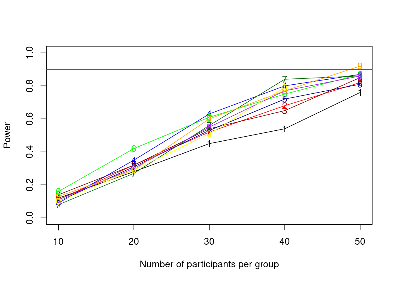
As we can see in this admittedly not very elegant plot, in which each line represents a number of songs, the power reaches the desired minimum of 90 percent at 50 participants listening to 90 songs.
Final words
That’s it. You should now be able to run power analysis for must of the mixed model situations that you might find yourself in. However, a few things are still missing for special cases but I feel like it is better to discuss them in some brief Appendices below, as they might not be relevant to everyone who is reading this:
Appendix A discusses how to speed up the power simulation.
While Appendix A might still be interesting to most, parallelization necessarily makes code more complicated and I did not want to convey the picture that it is something that must be done. If you find yourself in a situation where the simulation is taking very long, I still recommend reading this part.
Appendix B discusses how to extend designs to include factors with more than 2 levels and interactions.
Appendix B discusses how to include factors with more than two levels in the simulation as well as interactions with random effects. It contains two useful functions, an extension of the generate design function and a function to create the variance-covariance matrices that we created by hand thus far. I think these can be useful in many cases, so I recommend checking it out as well.
Appendix C discusses how to run a true-positive detection rate analysis (aka Bayesian Power Analysis) using the brms package.
Appendix C discusses how to simulate data the Bayesian way. Here, we use priors to specify our expected effects and can leave the rest to the model by just sampling from the prior. If you are using Bayesian analyses already, I recommend reading it, otherwise you should first get acquainted with Bayesian Analyses (which I would recommend as well) by reading, for example, the fantastic book Statistical Rethinking by Richard McElreath
I hope you found this tutorial useful and I are happy to hear your feedback and suggestions in comments or emails!
Appendices
Appendix A: Speeding up the simulation
As you might have noticed, mixed-effect model power simulations take much longer than the previous cases that we worked with. There are multiple things we could do to make this quicker.
1. Run a low-resolution simulation first
First, we could again have a low-resolution –> high resolution approach where we only try very few sample sizes in a first step and then move to a more fine-grained simulation.
2. Optimalize the code
Second, there are a few things in this code that are not yet as efficient as they could be.
For instance, saving the power and convergence info to the data-frame directly saves a few lines of code and extra objects, but it would be quicker to first save everything to vectors and then rbind() them to the data-frame.
As the data-frame is not too big here (only 500 rows with 2 columns) I would not expect too much of a speed-up here though.
Furthermore, we could change the simulation loop for the DV to an apply function, which should also save a few seconds in total.
Again, I do not expect huge speed ups here so this would be something to do if time is really a factor.
3. Parallelize the simulations
As you will probably know, modern computers usually have more than 1 CPU core, which means they can execute multiple tasks in parallel.
The current loop does not take advantage of that and only 1 CPU core will be occupied with running our simulation, while all the others (5 in my case, of which each can execute 2 tasks in parallel due to hyper-threading) are not helping out.
There are multiple ways in R on how to execute code in parallel.
The most elegant one is probably the future package.
However, I personally prefer a rather bulky old-school style using the foreach package, as it is “easy” to control a lot of different parameters there.
The greatest speed-up probably comes with parallelization which will cut down the execution time approximately by the number of cores (minus a constant that it takes R to create separate “sessions” for each core and report back to the main session afterwards). Let us have a look how to parallelize the above code.
The way foreach works, is basically that it runs a for-loop in parallel, so if you have 6 cores with 2 threads each you could run the first 12 threads in parallel1.
Here, I will make use of 10 out of my 12 threads to make sure my computer can also do some other stuff with the remaining 2 threads.
The syntax for foreach might look somewhat alien if you have not seen it before, so lets look at it step by step.
First, we have to create a so-called cluster which is basically an object containing information about the cores.
library(parallel)
library(foreach)
library(doRNG)
library(doParallel)

n_threads <- detectCores()-2
cl <- makeCluster(rep("localhost", n_threads), outfile="mylog.txt")
The detectCores() bit finds out how many cores there are on the machine.
The makeCluster bit creates a cluster called cl for 10 parallel workers, which is my number of threads n_threads minus the 2 threads I want to keep idle for other stuff.
The last bit in makeCluster, outfile = "mylog.txt", is creating a file, in which we will be able to check for possible errors, as parallel sessions are not able to print something to the console.
Instead, we will print the output to a file and open it in RStudio, where we can see a live-version of the file.
Next, as foreach basically creates a new R-session for each thread, it will be necessary that we export the necessary objects from our global session to the “workers” which is what these parallel sessions are called.
The part we want to parallelize is the for loop that does the simulations, so each of the workers needs all objects that have been created outside of the for-loop but are used within it.
For this we use the following syntax:
n <- 3 # we set n to 3 to start in the second row of the pp_song_mat for the parallel loop (see below)
clusterExport(cl, list("generate_design", "b0", "b1", "b2", "epsilon",  "sigma_u01", "sigma_w01", "is_singular", "is_nonconv", "pp_song_mat", "n"))
clusterEvalQ(cl, c(library("lme4"), library("MASS"), library("afex")))
registerDoParallel(cl)
ClusterExport is a function that exports objects from the global environment (like custom functions and variables) to the workers and clusterEvalQ runs certain r-code on the cluster so that we can use packages there.
Last, registerDoParallel(cl) tells that everything in a foreach loop should be run in parallel.
The only thing left is to change some stuff in the loop.
The loop below looks quite different from the previous one, which has to do with the fact that we have to use a workaround to not give up the flexible stopping that is provided with the while loop entirely, as foreach has no conditional stopping rules (as far as I know)2.
The first thing that changed is that, we make a new object called last_powers and last_powers_cleaned.
These will hold the powers of the last iteration of the foreach loop, i.e. of the last n_threads = 10 combinations of participant number and song number as specified in the rows of the pp_song_mat data-frame.
You can see it like this:
Just like above, we specify the combination of number of participants and songs in the pp_song_mat data frame.
Each row tells us how many participants and songs this simulation should have.
However, instead of trying one combination at a time, we try n_threads = 10 combinations at the same time - each of them on one processor core.
The cores operate completely independent from each other, such that the results are unknown to our main R-session until they are reported back from the so-called “workers” that run on each core.
To make our R-session aware of the results from the workers, we need to return the results to our R-session, which is what we do in the line with the return statement, where, just as above, we return the power, the number of singular models, the number of non-converging models, the number of skipped simulations due to 0 instrument players and the par_n parameter of each simulation to check whether the power that we retrieve is actually reported to the right row of the data-frame.
To understand the parallel loop, it helps to see the compare the structure to a regular loop:
# traditional for loop
for(par_n in next_n_group){
  ...
  last_powers <- (c(mean(p_vals < alpha), mean(na.omit(is_singular)), mean(na.omit(is_nonconv)), skips_at_n, par_n))
}

# parallel foreach loop
last_powers <- foreach(par_n = next_n_group) %dorng% {
  ...
  return(c(mean(p_vals < alpha), mean(na.omit(is_singular)), mean(na.omit(is_nonconv)), skips_at_n, par_n))
}
This might help to see how the approach is actually very similar, but just needs to be set up a bit differently.
The weird %dorng% thingy is a variation of the more understandable %doparallel% code, that we do not use here, as %dorng% allows us to set a seed and thereby make the simulation reproducible.
The rest of the code basically just makes sure that everything that we also saved above is stored in the right place by using the par_n index.
In the end, we save the outcome from the foreach loop to an object into pp_song_mat in our global R session, which gives us the same data-set above, containing the powers.
start_time <- Sys.time()

last_powers <- rep(-999, n_threads) # this one will be the output of the foreach loop
last_powers_cleaned <- rep(-999, n_threads) # this will be a cleaned object of the foreach output that we use for the while-loop
# n <- 3
next_n_group <- (n-1):(n+n_threads-2)


#### increasing sample size ####
set.seed(987654321)
while(all(last_powers_cleaned < power_crit)){


  #### increasing simulation number ####
  last_powers <- foreach(par_n = next_n_group) %dorng% {
  # for(par_n in next_n_group){

    skips_at_n <- 0
    is_singular <- c()
    is_nonconv <- c()

    for(sim in 1:n_sims){

      # make design-matrix
      tmp_dat <- generate_design(n_participants = pp_song_mat$participant[par_n], n_genres = 2,
                                 n_songs = pp_song_mat$song[par_n], prop_instrument = .20)
      tmp_dat$genre_pop <- ifelse(tmp_dat$genre == "pop", 1, -1)
      tmp_dat$instrument_yes <- ifelse(tmp_dat$instrument == "yes", 1, -1)

      #### making sure that there is at least 1 instrument player in the data (otherwise the model does cannot be fit) ####
      if (mean(tmp_dat$instrument_yes) != -1){

        unique_songs <- unique(tmp_dat$song)
        tmp_dat$genre <- factor(tmp_dat$genre)
        tmp_dat$instrument <- factor(tmp_dat$instrument, levels = c("yes", "no"))

        # make random effect matrices
        U01 <- mvrnorm(length(unique(tmp_dat$participant)),c(0,0),sigma_u01)
        W01 <- mvrnorm(length(unique(tmp_dat$song)),c(0,0),sigma_w01)

        #### create the DV ####
        for(i in 1:nrow(tmp_dat)){
          tmp_dat$liking[i] <- rnorm(1,
                                   b0+ # fixed intercept (average liking)
                                     U01[tmp_dat$participant[i], 1] + # random intercept for participants
                                   W01[which(unique_songs == tmp_dat$song[i]), 1] + # random intercept term for song
                                   (b1+ # fixed effect of genre (which is 0)
                                      U01[tmp_dat$participant[i], 2]) # random slope for genre across participants
                                   *tmp_dat$genre_pop[i] # for each row whether its pop or rock
                                   +(b2+ # fixed effect of instrument
                                       W01[which(unique_songs == tmp_dat$song[i]), 2])
                                   *tmp_dat$instrument_yes[i]# random slope for instrument across songs
                                   , epsilon) # residual SD

        }

        #### fit model ####
        tmp_lmem <- suppressMessages(mixed(liking ~ genre + instrument
                                           + (1 + genre | participant) + (1 + instrument | song),
                                           tmp_dat, method = "S", control = lmerControl(optimizer = "bobyqa"), progress = F))

        p_vals[sim] <- tmp_lmem$anova_table$`Pr(>F)`[2] # extract p-value for instrument


        #### check for model convergence and singular fits ####
        is_singular[sim] <- ifelse(max(grepl("singular", tmp_lmem[["full_model"]]@optinfo[["conv"]][["lme4"]][["messages"]]
                                         , fixed = T)) > 0, 1, 0)
        is_nonconv[sim] <- ifelse(max(grepl("failed", tmp_lmem[["full_model"]]@optinfo[["conv"]][["lme4"]][["messages"]]
                                        , fixed = T)) > 0, 1, 0)

      } else { # this happens if there is not a single instrument player in our sample

        p_vals[sim] <- 1 # set p-value to 1 manually
        skips_at_n <- skips_at_n+1 # update number of skipped simulations because of 0 instrument players
        # print("skipping sim because no single instrument player")

      }
    }
    return(c(mean(p_vals < alpha), mean(na.omit(is_singular)), mean(na.omit(is_nonconv)), skips_at_n, par_n))
    # test_v <- (c(mean(p_vals < alpha), mean(na.omit(is_singular)), mean(na.omit(is_nonconv)), skips_at_n, par_n))
  } # end of single-n simulation for-loop
  #### calculat epower and print a message to see our progress

  for(ser_n in 1:n_threads){
    last_powers_cleaned[ser_n] <- last_powers[[ser_n]][1] # add the power to the cleaned while-loop check
    pp_song_mat$power[next_n_group[ser_n]] <- last_powers[[ser_n]][1] # add power to data-frame
    pp_song_mat$p_singular[next_n_group[ser_n]] <- last_powers[[ser_n]][2] # save proportion of singular models to pp_song_mat
    pp_song_mat$p_nonconv[next_n_group[ser_n]] <- last_powers[[ser_n]][3] # save proportion of non-converging models to pp_song_mat
    pp_song_mat$skips_at_n[next_n_group[ser_n]] <- last_powers[[ser_n]][4] # add this number to pp_song_mat so we can have a look at it later
    pp_song_mat$control_row[next_n_group[ser_n]] <- last_powers[[ser_n]][5] # add this a a check whether the parallel outputs are saved at the right row of the data-frame
  }
    print("################################################")
    print(paste0("current highest sample-size in block: ", pp_song_mat$participant[n+n_threads-2],
                 " with ", pp_song_mat$song[n+n_threads-2], " songs"))
    print(paste0("highest power from last block: ", max(last_powers_cleaned)))
    print(Sys.time() - start_time)
    n <- n+n_threads # increase n for next iteration
    next_n_group <- (n-1):(n+n_threads-2)
}
## [1] "################################################"
## [1] "current highest sample-size in block: 10 with 100 songs"
## [1] "highest power from last block: 0.14"
## Time difference of 1.417292 mins
## [1] "################################################"
## [1] "current highest sample-size in block: 20 with 100 songs"
## [1] "highest power from last block: 0.38"
## Time difference of 5.208043 mins
## [1] "################################################"
## [1] "current highest sample-size in block: 30 with 100 songs"
## [1] "highest power from last block: 0.63"
## Time difference of 11.91706 mins
## [1] "################################################"
## [1] "current highest sample-size in block: 40 with 100 songs"
## [1] "highest power from last block: 0.8"
## Time difference of 22.34133 mins
## [1] "################################################"
## [1] "current highest sample-size in block: 50 with 100 songs"
## [1] "highest power from last block: 0.92"
## Time difference of 37.00339 minsAppendix B: Factors with more than 2 levels
So far, we only used factors with 2 levels, where it was easy to make a variable that codes the levels as numbers (i.e. 1 for pop and -1 for rock so far). However, as soon as factors have more than 2 levels, things get a little more complicated as we have to use not one but two contrasts in order to make all relevant comparisons.
Thus, for the simulation we need 2 variables in the data frame for a factor with 3 levels, and 4 variables with a factor of 5 levels etc. Each of these variables needs it’s own effect size and random effect specified.
The code below shows how we can do this with the example above, now adding a classic factor to the genre variable.
generate_design <- function(n_participants, n_genres, n_songs, prop_instrument = .20, genre_names = c()){
  # we have a new genre_name argument here to assign factor levels dynamically.
  design_matrix <- expand.grid(participant = 1:n_participants, genre = 1:n_genres, song = 1:n_songs)
  design_matrix$song <- paste0(design_matrix$genre, "_", design_matrix$song)
  # NOTE THAT I DELETED THE LINE THAT ASSIGNED ROCK POP HERE TO MAKE THE FUNCTION MORE FLEXIBLE
  instrument_players <- sample(c("yes", "no"), n_participants, prob = c(prop_instrument, (1-prop_instrument)), replace = T) # sample whether people play instrument
  for(i in 1:nrow(design_matrix)){ # grant people the ability to play instrument
    design_matrix$instrument[i] <- instrument_players[design_matrix$participant[i]]
    design_matrix$genre[i] <- genre_names[as.integer(design_matrix$genre[i])]
  }

  return(design_matrix)
}

set.seed(1)
data4 <- generate_design(n_participants = 10, n_genres = 3, n_songs = 20, prop_instrument = .20, genre_names = c("pop", "rock", "classic")) # we add the classic genre

# assign levels to to original variables
data4$genre <- factor(data4$genre, levels = c("pop", "rock", "classic"))
data4$instrument <- factor(data4$instrument, levels = c("yes", "no"))
The code above changed the generate_design function slightly, so that we can now use it to create as many factor levels as we want for the genre variable.
Next, I created a function that allows us to add factor-contrast variables to the data set automatically.
This is what we did manually before when creating the genre_pop and instrument_yes variables.
Now the function will take care of that for us and create these variables automatically by using the factor levels from the variable that we supply.
add_contrast_vars <- function(data, var){

  cm <- contrasts(data[,var]) # extract contrast matrix from variable
  for(i in 1:length(cm[1,])){ # for each contrast
    cm_var <- cm[, i]  # take the current values for this contrast
    cm_var_name <- paste0(var, "_", names(which(cm_var == 1))) # get the name of the variable coded as 1
    if((cm_var_name %in% names(data)) == FALSE){ # if this is the first time we use this on this data frame
      for(i in 1:nrow(data)){ # for each row
          data[i, cm_var_name] <- cm_var[names(cm_var) == data[i, var]] # assign the value for this contrast
      }
    }
  }
  return(data) # return updated data
}

data4 <- add_contrast_vars(data4, "genre")
data4 <- add_contrast_vars(data4, "instrument")
str(data4)
## 'data.frame': 600 obs. of 7 variables:
## $ participant : int 1 2 3 4 5 6 7 8 9 10 ...
## $ genre : Factor w/ 3 levels "pop","rock","classic": 1 1 1 1 1 1 1 1 1 1 ...
## $ song : chr "1_1" "1_1" "1_1" "1_1" ...
## $ instrument : Factor w/ 2 levels "yes","no": 2 2 2 1 2 1 1 2 2 2 ...
## $ genre_pop : num 1 1 1 1 1 1 1 1 1 1 ...
## $ genre_rock : num 0 0 0 0 0 0 0 0 0 0 ...
## $ instrument_yes: num -1 -1 -1 1 -1 1 1 -1 -1 -1 ...
## - attr(*, "out.attrs")=List of 2
## ..$ dim : Named int [1:3] 10 3 20
## .. ..- attr(*, "names")= chr [1:3] "participant" "genre" "song"
## ..$ dimnames:List of 3
## .. ..$ participant: chr [1:10] "participant= 1" "participant= 2" "participant= 3" "participant= 4" ...
## .. ..$ genre : chr [1:3] "genre=1" "genre=2" "genre=3"
## .. ..$ song : chr [1:20] "song= 1" "song= 2" "song= 3" "song= 4" ...We now have 2 new variables in the data frame genre_pop and genre_rock, that are the numeric representations of the respective factor levels.
We can use those and put them into the regression equation like we did before.
To add random effects, we also have to adjust the random effect variance-covariance matrix to include the random effects for each contrast now.
Filling in the variance-covariance matrix might become more difficult as the matrix keeps growing with more factor levels.
It might help to think of it as a k by k matrix, where k is the the number of factor contrasts + 1, that is filled column-wise from left to right and top to bottom.
In this matrix, the intercept variance must have column number 1, and the contrasts will have the other row and column numbers, such that on the diagonal there are always the variances. The covariances are in between such that in row 2, column 3, there will, for instance, be the covariance of contrast 1 with contrast 2.
As is usual for variance-covariance matrices, each covariance will be in there twice as the part above and below the diagonal contain the same information. It might make sense to fill the matrix with words first to see whether everything ends up on the right spot:
sigma_u01 <- matrix(c("col1/row1: variance of random intercept",
                      "col1/row2: intercept-pop covariance",
                      "col1/row3: intercept-rock covariance",
                      "col2/row1: intercept-pop covariance",
                      "col2/row2: pop variance",
                      "col2/row3: pop-rock covariance",
                      "col3/row1: intercept-rock covariance",
                      "col3/row2: pop-rock covariance",
                      "col3/row3: rock variance"
                      ), ncol = 3) #c3/r3: rock variance

sigma_u01
## [,1]
## [1,] "col1/row1: variance of random intercept"
## [2,] "col1/row2: intercept-pop covariance"
## [3,] "col1/row3: intercept-rock covariance"
## [,2]
## [1,] "col2/row1: intercept-pop covariance"
## [2,] "col2/row2: pop variance"
## [3,] "col2/row3: pop-rock covariance"
## [,3]
## [1,] "col3/row1: intercept-rock covariance"
## [2,] "col3/row2: pop-rock covariance"
## [3,] "col3/row3: rock variance"Now we can take this and fill in the numbers.
set.seed(1)
b0 <- 75
b1a <- -2 # difference between pop and grand mean
b1b <- 7 # difference between rock and grand mean
b2 <- 2.5 # the instrument effect
sd_u0 <- sqrt(11.25)
epsilon <- sqrt(56.25-11.25)
sd_u1a <- 5 # random slope of pop
sd_u1b <- 7 # random slope of rock
corr_u01a <- -.20 # random correlation between intercept and pop slope
corr_u01b <- .20 # random correlation between intercept and rock slope
corr_u1a1b <- .50 # random correlation between pop and rock slopes

sigma_u01 <- matrix(c(sd_u0^2, # col1/row1: variance of random intercept
                      sd_u0*sd_u1a*corr_u01a, #c1/r2: intercept-pop covariance
                      sd_u0*sd_u1b*corr_u01b, #c1/r3: intercept-rock covariance
                      sd_u0*sd_u1a*corr_u01a, #c2/r1: intercept-pop covariance
                      sd_u1a^2, # c2/r2: pop variance
                      sd_u1a*sd_u1b*corr_u1a1b, #c2/r3: pop-rock covariance
                      sd_u0*sd_u1b*corr_u01b, #c3/r1: intercept-rock covariance
                      sd_u1a*sd_u1b*corr_u1a1b, #c3/r2: pop-rock covariance
                      sd_u1b^2), ncol = 3) #c3/r3: rock variance

sigma_u01
## [,1] [,2] [,3]
## [1,] 11.250000 -3.354102 4.695743
## [2,] -3.354102 25.000000 17.500000
## [3,] 4.695743 17.500000 49.000000All the numbers end up in the right spot, as you can see (by the way I just used some random numbers here for the parameters as this is merely for demonstration).
Now we can create the random effect distributions again and put the contrast variables into the regression equation to simulate the DV.
U01 <- mvrnorm(length(unique(data4$participant)),c(0,0, 0),sigma_u01)

sd_w0 <- sqrt(11.25)/2
sd_w1 <- sd_w0/4
corr_w01 <- .10
sigma_w01 <- matrix(c(sd_w0^2, sd_w0*sd_w1*corr_w01, sd_u0*sd_w1*corr_u01, sd_w1^2), ncol = 2)
W01 <- mvrnorm(length(unique(data4$song)),c(0,0),sigma_w01)


unique_songs <- unique(data4$song)
for(i in 1:nrow(data4)){
  data4$liking[i] <- rnorm(1,
                           b0+ # fixed intercept (average liking)
                             U01[data4$participant[i], 1] + # random intercept for participants
                           W01[which(unique_songs == data4$song[i]), 1] + # random intercept term for song
                           (b1a+ # fixed effect of genre (which is 0)
                              U01[data4$participant[i], 2]) # random slope for genre across participants
                           *data4$genre_pop[i]  # for each row whether its pop
                           +(b1b+ # fixed effect of genre (which is 0)
                              U01[data4$participant[i], 3]) # random slope for genre across participants
                           *data4$genre_rock[i]  # for each row whether its rock
                           +(b2+ # fixed effect of instrument
                               W01[which(unique_songs == data4$song[i]), 2])
                           *data4$instrument_yes[i]# random slope for instrument across songs
                           , epsilon) # residual SD

}


lmem8 <- lmer(liking ~ genre + instrument + (1 + genre | participant) + (1 + instrument | song), data4, control = lmerControl(optimizer = "bobyqa"))
summary(lmem8)
## Linear mixed model fit by REML. t-tests use Satterthwaite's method [
## lmerModLmerTest]
## Formula: liking ~ genre + instrument + (1 + genre | participant) + (1 +
## instrument | song)
## Data: data4
## Control: lmerControl(optimizer = "bobyqa")
##
## REML criterion at convergence: 4133.3
##
## Scaled residuals:
## Min 1Q Median 3Q Max
## -2.9631 -0.6344 -0.0373 0.6788 3.7243
##
## Random effects:
## Groups Name Variance Std.Dev. Corr
## song (Intercept) 1.014 1.007
## instrument1 1.056 1.028 0.69
## participant (Intercept) 15.925 3.991
## genre1 16.270 4.034 -0.83
## genre2 35.862 5.989 -0.36 0.46
## Residual 50.258 7.089
## Number of obs: 600, groups: song, 60; participant, 10
##
## Fixed effects:
## Estimate Std. Error df t value Pr(>|t|)
## (Intercept) 74.5054 1.3514 6.6116 55.133 0.000000000469 ***
## genre1 -3.1157 1.3472 9.0210 -2.313 0.04597 *
## genre2 8.1687 1.9427 9.0931 4.205 0.00224 **
## instrument1 1.3976 0.9217 8.5766 1.516 0.16542
## ---
## Signif. codes: 0 '***' 0.001 '**' 0.01 '*' 0.05 '.' 0.1 ' ' 1
##
## Correlation of Fixed Effects:
## (Intr) genre1 genre2
## genre1 -0.730
## genre2 -0.327 0.387
## instrument1 0.277 0.005 -0.002As you can see, the only thing that changed here compared to previous versions is that we split up the genre effect into b1a for the effect of pop and b1b for the effect of rock.
Both of them get a line in the simulation code, with the U01[data4$participant[i], 2] and U01[data4$participant[i], 3] referring to the random effect distribution of pop and rock respectively.
Adding an interaction
What if we would like to add the genre by instrument interaction here?
As this is a within-between interaction, there will be no random effects associated with this interaction.
Therefore, we can add it just as we did earlier in part 3 of this tutorial.
For instance the b1ab2 effect size refers to how much bigger we expect the difference of pop music from the grand mean to be for people who do play an instrument compared to people who do not play an instrument.
b1bb2 Has the same interpretation for rock music.
b1ab2 <- -3
b1bb2 <- 12

unique_songs <- unique(data4$song)
for(i in 1:nrow(data4)){
  data4$liking[i] <- rnorm(1,
                           b0+ # fixed intercept (average liking)
                             U01[data4$participant[i], 1] + # random intercept for participants
                           W01[which(unique_songs == data4$song[i]), 1] + # random intercept term for song
                           (b1a+ # fixed effect of genre (which is 0)
                              U01[data4$participant[i], 2]) # random slope for genre across participants
                           *data4$genre_pop[i]  # for each row whether its pop
                           +(b1b+ # fixed effect of genre (which is 0)
                              U01[data4$participant[i], 3]) # random slope for genre across participants
                           *data4$genre_rock[i]  # for each row whether its rock
                           +b1ab2*data4$genre_pop[i]*data4$instrument_yes[i] # pop*instrument interaction
                           +b1bb2*data4$genre_rock[i]*data4$instrument_yes[i] # rock*instrument interaction
                           +(b2+ # fixed effect of instrument
                               W01[which(unique_songs == data4$song[i]), 2])
                           *data4$instrument_yes[i]# random slope for instrument across songs
                           , epsilon) # residual SD

}


lmem9 <- lmer(liking ~ genre * instrument + (1 + genre * instrument | participant) + (1 + instrument | song), data4, control = lmerControl(optimizer = "bobyqa"))
## boundary (singular) fit: see ?isSingularsummary(lmem9)## Linear mixed model fit by REML. t-tests use Satterthwaite's method [
## lmerModLmerTest]
## Formula:
## liking ~ genre * instrument + (1 + genre * instrument | participant) +
## (1 + instrument | song)
## Data: data4
## Control: lmerControl(optimizer = "bobyqa")
##
## REML criterion at convergence: 4100
##
## Scaled residuals:
## Min 1Q Median 3Q Max
## -2.9706 -0.6655 0.0055 0.6835 3.2152
##
## Random effects:
## Groups Name Variance Std.Dev. Corr
## song (Intercept) 1.3606443 1.16647
## instrument1 0.0003257 0.01805 1.00
## participant (Intercept) 5.4140813 2.32682
## genre1 12.3449699 3.51354 -0.56
## genre2 24.3080763 4.93032 0.11 0.65
## instrument1 15.0023384 3.87329 0.61 -0.87 -0.33
## genre1:instrument1 14.3134080 3.78331 -0.58 0.94 0.58 -0.91
## genre2:instrument1 12.6011017 3.54980 -0.70 0.82 0.20 -0.90
## Residual 48.9195750 6.99425
##
##
##
##
##
##
##
##
## 0.89
##
## Number of obs: 600, groups: song, 60; participant, 10
##
## Fixed effects:
## Estimate Std. Error df t value Pr(>|t|)
## (Intercept) 74.0413 1.7531 2.6051 42.235 0.000091 ***
## genre1 -1.6228 2.1450 2.1525 -0.757 0.5234
## genre2 8.2713 2.2298 3.3231 3.709 0.0286 *
## instrument1 -0.1673 1.7466 2.5670 -0.096 0.9307
## genre1:instrument1 0.2586 2.1344 2.1105 0.121 0.9141
## genre2:instrument1 11.9038 2.2196 3.2632 5.363 0.0102 *
## ---
## Signif. codes: 0 '***' 0.001 '**' 0.01 '*' 0.05 '.' 0.1 ' ' 1
##
## Correlation of Fixed Effects:
## (Intr) genre1 genre2 instr1 gnr1:1
## genre1 -0.784
## genre2 -0.485 0.762
## instrument1 0.757 -0.769 -0.503
## gnr1:nstrm1 -0.770 0.943 0.750 -0.791
## gnr2:nstrm1 -0.504 0.750 0.542 -0.489 0.775
## optimizer (bobyqa) convergence code: 0 (OK)
## boundary (singular) fit: see ?isSingularAs you can see above the only thing left to do then is to multiply the effect by the respective indicators for each row identifying the genre and whether the person plays an instrument for each row.
For b1ab2 we multiply by the genre_pop contrast variable, and for b1bb2 we use the genre_rock variable.
For example, for a row of a person that does play an instrument and a song that is a pop song, the value will be:
b1ab2*data4$genre_pop[i]*data4$instrument_yes[i] = -3*1*1 = -3.
Extending Random-Effect matrices
If the interaction would be fully within participants and we would like to add random effects, they can be added to the random effect matrix in the exact same way that we added the 2nd contrast for genre above.
The matrix just needs to grow by two additional row and column (i.e. have 6x6 = 36 total entries).
the first 3 columns would contain the same information as before in the first 3 rows and 3 additional rows for the main effect of instrument and the genre_pop*instrument_yes and genre_rock*instrument_yes interactions respectively.
Columns 4, 5 and 6 would contain the variances and covariances of those additional variables.
that now also contain the variance of the random effect for the main effect of instrument, as well as interaction and the covariances with the random intercept of participant and the random slopes of genre_pop and genre_rock.
As this can be very time-consuming, I created a function make_vcov_matrix that can help with creating the random effect matrices.
As demonstrated below, you can pass to it the parameters and the correlations between the parameters (in this case 15 correlation for the 6 effects (6^2-6)/2).
sd_u0 <- 1 # random intercept
sd_u1a <- 2 # random slope of pop
sd_u1b <- 3 # random slope of rock
sd_u2 <- 4 # random slope of instrument
sd_u1a2 <- 5 # random slope of pop X instrument interaction slopes
sd_u1b2 <- 6 # random slope of rock X instrument interaction slopes

corr_u01a <- .01 # random correlation between intercept and pop slope
corr_u01b <- .02 # random correlation between intercept and rock slope
corr_u02 <- .03 # random correlation between intercept and instrument slope
corr_u01a2 <- .04 # random correlation between intercept and pop X instrument interaction slopes
corr_u01b2 <- .05 # random correlation between intercept and rock X instrument interaction slopes

corr_u1a1b <- .06 # random correlation between pop and rock slopes
corr_u1a2 <- .07 # random correlation between pop and instrument slopes
corr_u1a1a2 <- .08 # random correlation between pop and pop X instrument interaction slopes
corr_u1a1b2 <- .09 # random correlation between pop and rock X instrument interaction slopes

corr_u1b2 <- .10 # random correlation between rock and instrument slopes
corr_u1b1a2 <- .11 # random correlation between rock and pop X instrument interaction slopes
corr_u1b1b2 <- .12 # random correlation between rock and rock X instrument interaction slopes

corr_u21a2 <- .13 # random correlation between instrument and pop X instrument interaction slopes
corr_u21b2 <- .14 # random correlation between instrument and rock X instrument interaction slopes

corr_u1a21b2 <- .15 # random correlation between pop X instrument interaction and rock X instrument interaction slopes

pars <- c(sd_u0, sd_u1a, sd_u1b, sd_u2, sd_u1a2, sd_u1b2)

corrs <- c(corr_u01a, corr_u01b, corr_u02, corr_u01a2, corr_u01b2,
           corr_u1a1b, corr_u1a2, corr_u1a1a2, corr_u1a1b2,
           corr_u1b2, corr_u1b1a2, corr_u1b1b2,
           corr_u21a2, corr_u21b2,
           corr_u1a21b2
           )


make_vcov_matrix <- function(pars = c(), corrs = c()){

  # make empty square matrix of size length(pars)
  m <- matrix(rep(NA), nrow = length(pars), ncol = length(pars))
  k_low <- 1 # counter for below diagonal matrix
  k_high <- 1 # counter for above diagonal matrix

  # the loop basically iterates over the columns and rows and fills in the variances and covariances in both diagonals of the matrix
  for(col in 1:ncol(m)){
    for(row in 1:nrow(m)){
      if(col == row){
        m[row, col] <- pars[col]*pars[row]
      } else {
        if(col < row){
          m[row, col] <- pars[col]*pars[row]*corrs[k_low]
          k_low <- k_low+1
        } else {
          m[row, col] <- pars[col]*pars[row]*corrs[k_high]
          k_high <- k_high+1
        }

      }
    }

  }

  return(m) # return the filled-in matrix

}

sigma_u <- make_vcov_matrix(pars, corrs)

U <- mvrnorm(length(unique(data4$participant)),rep(0, length(pars)),sigma_u)
Note that the order that you pass the arguments to the function should be the same order that you will use it in the regression-equation simulation approach.
This is, whatever effect you enter the function first (e.g. the random intercept), can be assessed later as U[data$participant[i], 1] for example, meaning that the first effect will be in the first column of U and the second effect in the second column etc.
The correlation need to be entered in the following order:
- E1 x E2, E1 x E3, E1 x E4, E1 x E5, E1 x E6
- E2 x E3, E2 x E4 ….
which in terms of the example is
- intercept x genre_pop, intercept x genre_rock, intercept x instrument, intercept x genre_pop:instrument, intercept x genre_rock:instrument
- genre_pop x genre_rock, genre_pop x instrument …..
Thus, in terms of the variance-covariance matrix this corresponds to entering the correlations column-wise for the lower diagonal of the matrix.
Appendix C: Bayesian Data Simulation with brms
The Bayesian approach to power simulation - or more technically correct True-Positive Rate simulation as power is not really a Bayesian concept - is a little different from what we did above.
We will still generate a design matrix but instead of simulating the outcome variable using rnorm or other simulation functions, we can make use of the fact that Bayesian models have prior information as a part of the model itself.
This means that when running a simulation, we can tell the model our expectations by using them as priors, and then tell the model to simulate those priors, which will give us the expected outcome variables.
This may sound weird but the nice thing about it is that we do not need imitate the model by writing the model formula ourselves in the simulation but can just use the formula from the model directly.
I assume that you already know brms at this point, so I will not go into detail too much and just give a demonstration on how to simulate data using brms.
First we will define the prior, setting the parameters for the simulation.
brms does not really support setting random correlations independently for each random effect so we will not do this here.
Afterwards we will generate a design, just like above, and fit a brms model that only samples from the prior. This model will serve as our “simulation engine” that will generate the dependent variable predictions.
When specifying the priors, the class argument sets which kind of effect it is about (intercept, b = fixed or sd = random) and coef defines the name of the parameter (the 1 is added here (e.g. instrument1) because of the contrast coding).
The group in the random effects terms specifies which grouping factor the effect refers to.
What we called epsilon before, i.e. the residual variation, is now called sigma.
Note that we defined all parameters as normal distributions with a standard deviation of 1.
We could also decrease the standard deviation further, but it does not really matter here, as long as the standard deviations are reasonably small.
library(brms)

priors_sim <- c(set_prior("normal(75,1)", class = "Intercept"),
                set_prior("normal(0,1)", class = "b", coef = "genre1"),
                set_prior("normal(2.5,1)", class = "b", coef = "instrument1"),
                set_prior("normal(3.354102,1)", class = "sd", coef = "Intercept", group = "participant"),
                set_prior("normal(5,1)", class = "sd", coef = "genre1", group = "participant"),
                set_prior("normal(1.677051,1)", class = "sd", coef = "Intercept", group = "song"),
                set_prior("normal(0.4192628,1)", class = "sd", coef = "instrument1", group = "song"),
                set_prior("normal(6.708204,1)", class = "sigma"))

init_dat <- generate_design(n_participants = 100, n_genres = 2,
                               n_songs = 50, prop_instrument = .20, genre_names = c("pop", "rock"))

init_dat$liking <- rep(-999)

brm_prior <- brm(liking ~ genre + instrument + (1 + genre | participant) + (1 + instrument | song), init_dat, cores = 4, chains = 4, sample_prior = "only", prior = priors_sim)
## Compiling Stan program...## Start samplingThe next step is to predict values of the outcome variable given our simulation parameters that we specified in the prior.
We do this in the code below by using the predict function.
Importantly, we need to set the summary=FALSE argument to tell brms to not summarize the predictions but instead give us the raw predicted values.
We add these values to the data frame and fit a new model now that will test whether these predictions show a credible effect of the variable of interest.
For this we use a custom function called brm_postprop that will provide the proportion of posterior density that is smaller or larger than zero.
init_dat$liking <- predict(brm_prior, newdata = init_dat, summary=FALSE, nsamples=1)[1,]

brm_post <- brm(liking ~ genre + instrument + (1 + genre | participant) + (1 + instrument | song), init_dat, cores = 4, chains = 4)
## Compiling Stan program...## Start sampling# compute posterior probability > or < 0 for parameter.
brm_postprop <- function(brm_fit, pars, direction = c("<", ">")){
post_samples <- c(posterior_samples(brm_fit, pars = pars))[[1]]
if (direction == "<") {
postprob <- mean(post_samples < 0)
} else if (direction == ">") {
postprob <- mean(post_samples > 0)
} else {
warning("direction must be either '<' or '>'")
}
return(postprob)
}
postprop <- brm_postprop(brm_post, "instrument1", direction = "<")
postprop## [1] 0.12025The above code shows everything that we need to do to simulate data in brms.
- Fit the prior model
- predict the outcome
- fit the post model to see whether the result is credible.
We can use this to do a power analysis by performing the second code chunk here in a loop, just as we did above and test the proportion of posterior probabilities that are smaller than the desired alpha-value.
Specifically, you should run the code as shown above and fit the first brm_post model outside of the loop, such that you can refit the models in the loop using the brms::update function, to prevent the model from being recompiled every iteration of the loop:
while(pp_song_mat$power[n] < power_crit){
  n <- n+1 # increase n for next iteration
  skips_at_n <- 0 # initialize counter for how many trials were skipped

  #### increasing simulation number ####
  for(i in 1:n_sims){

    # make design-matrix
    tmp_dat <- generate_design(n_participants = pp_song_mat$participant[n], n_genres = 2,
                               n_songs = pp_song_mat$song[n],
                               prop_instrument = .20, genre_names = c("pop", "rock"))
    tmp_dat$liking <- predict(brm_prior, newdata = tmp_dat, summary=FALSE, nsamples=1,
                              allow_new_levels =TRUE)[1,]
    brm_tmp <- update(brm_post, newdata = tmp_dat)
    postprops[i] <- brm_postprop(brm_tmp, "instrument1", direction = "<")
  }
  pp_song_mat$power[n] <- mean(postprops < alpha)

}
I do not run this here as it would take too long, but as you can see the structure of the loop is in principle the same as in the frequentist case, such that you can just replace the relevant code components, even in the parallel case.
Footnotes
Running more than 6 sessions on a 6 core / 12 thread processor will not increase the speed linearly anymore, as using both threads per core will decrease the speed per parallel session. In the end, 12 sessions might still be faster than 6 sessions though, but from my personal experience it does not matter that much.↩︎
In fact, this parallel loop is not super optimal, as the threads that have already finished simulating for a given sample size need to wait for the other threads to be done before moving on to the next blocks of n’s. That is not really nice but it is good enough to still provide some speed-up without giving up the flexibility that comes with the optional stopping of the while loop, which would otherwise not be possible, had we just used foreach to iterate over the participant number + song number combination directly.↩︎