Power Analysis by Data Simulation in R - Part II
Part II - simulating groups and powering t-tests
The Power Analysis by simulation in R for really any design - Part II
This is Part II of my tutorial on how to do power-analysis by simulation. In Part I, we saw how to do a simulation for a simple toy-example with a coin-toss. In this part, we will use a more realistic problem that we might encounter in our daily research life and see how to simulate the power for these designs. By looking at how to do power-simulation for the independent-samples t-test and the paired t-test we will learn how to simulate normal-distributions, how to specify their effect-sizes, in terms of \(Cohen's\ d\). Moreover, we simulate correlated (i.e. multivariate) normal distributions in cases where we have correlated observations (e.g. paired-sample t-test). This will be an important tool for later parts of this tutorial.
In part III of this tutorial we will learn how we can conceptualize basically any design as a linear model and thereby be very flexible in our power analysis. In part IV we will learn how to apply this technique to complicated designs such as linear mixed-effects models and generalized mixed-effects models.
Simulating a between-subjects t-test
Let’s get to it.
The first thing we will need again in our simulation is one of the implemented simulation functions in R (those that let R run theoretical experiments for us), but this time it is not rbinom as we are not working with coin-flips but rnorm - the simulation function for the normal distribution.
Let’s have a short look at that function as we will keep working with it throughout the tutorial.
rnorm(n, mean, sd) takes three arguments, a sample-size n, a mean and a standard-deviation sd.
By specifying these values, we can sample random ‘people’ (or observations) that are participating in our simulated experiments.
Imagine, for example, that we have an intervention study in which we have a treatment group and a control group.
We can easily simulate both groups with rnorm but what should the means and sds of the groups be?
There are two ways we can approach this.
- We could think about what group means we expect in our given case and what we expect the spread of the groups to be on the measurment scale that we are working with. For example, if we use a 40-point scale for a clinical test we might know that a group with deficiencies on the thing that we measure would probably score around 10 points and that almost everyone from that group would score lower than 20 points. This statement (most people score around 10, almost everyone scores lower than tified as normal distribution with a mean of 10 and a standard-deviation of 5. In this case only 2.5% of the values (i.e. the values outside the 95% CI) will be higher than 20.
- In a new research project, we might not be able or willing to to make these statements. In this case, by making some extra assumptions, we can fall back to the approach that we also use in power-calculation software in most cases and define a standardized effect size that we can use to simulate data rather than defining the group means and standard-deviations directly.
I personally try to go with the first approach whenever possible, as I think that in many cases we know more about what we expect from our data than we think, even in new projects. Even if we do not know a lot about our data, we might still try out different assumptions (i.e. means and sds) for the groups in our simulation to see what power we would get for each of them. This way, we can make informed decisions about our sample size that are more nuanced than the one in which we just assume a standardized effect size and see what sample-size it implies and are forced to think harder about our data - something that might seem difficult and annoying at first, but is extremely useful and eduucational. Another advantage of specifying the groups directly is that we can do this for any arbitrarily complex design where standardized effect sizes are often difficult to calculate.
This said, for the cases where we might really not be willing to specify groups directly, and because it allows me to demonstrate some other interesting points, in this part I will discuss how we can use standardized effect-sizes in our simulation. In part III and IV however, we will always specify effects on the raw scale.
If we were using GPower now, we would most likely just fill in a difference between groups in \(Cohen's\ d\) and be done with it.
We could of course also follow this approac in a simulation by defining the groups based on the implied \(Cohen's\ d\).
For instance, we can just assume that group 1 as rnorm(n, 1,2).
Now, following from the formula for Cohen’s d:
\[Cohen's\ d = \frac{(M_1 - M_2)}{pooled \ sd}\]
where
\[pooled\ sd = \sqrt\frac{(sd_1^2+sd_2^2)}{2}\]
and adhering to the student t-test assumption of equal variances we can fill in the pooled sd formula above as
\[pooled\ sd = \sqrt\frac{(2^2+2^2)}{2} = 2\]
to get a \(Cohen's\ d\) of .50:
\[Cohen's\ d = \frac{(1 - 0)}{2} = 0.5\]
To get any other value for \(Cohen's\ d\) we can just change the pooled sd value to whatever we want. More generally, we want to solve the equation above for the pooled sd after specifying any \(Cohen's\ d\), e.g.:
\[0.5= \frac{(1 - 0)}{pooled\ sd}\]
We can solve an equation like that with R’s somewhat unintuitive solve function like this:
solve(0.5,1) # cohens d of .5## [1] 2solve(0.25,1) # cohens d of .25## [1] 4solve(2,1) # cohens d of 2## [1] 0.5giving us three examples of how we would need to specify pooled sd to arrive at a particular \(Cohen's\ d\).
Thus, if we want to do a t-test with two simulated groups and a cohen’s d of 0.5 we can simulate two groups of a particular sample-size by using the rnorm function.
Let’s say we have 30 participants in each group.
set.seed(1234)
group1 <- rnorm(30, 1, 2)
group2 <- rnorm(30, 0, 2)
We can visualize the groups that we got in a plot like this:
hist(group1, col = "#addd8e", breaks = 10, main = "Histogram of both groups", xlab = "")
hist(group2, add = TRUE, breaks = 10, col= "#31a354")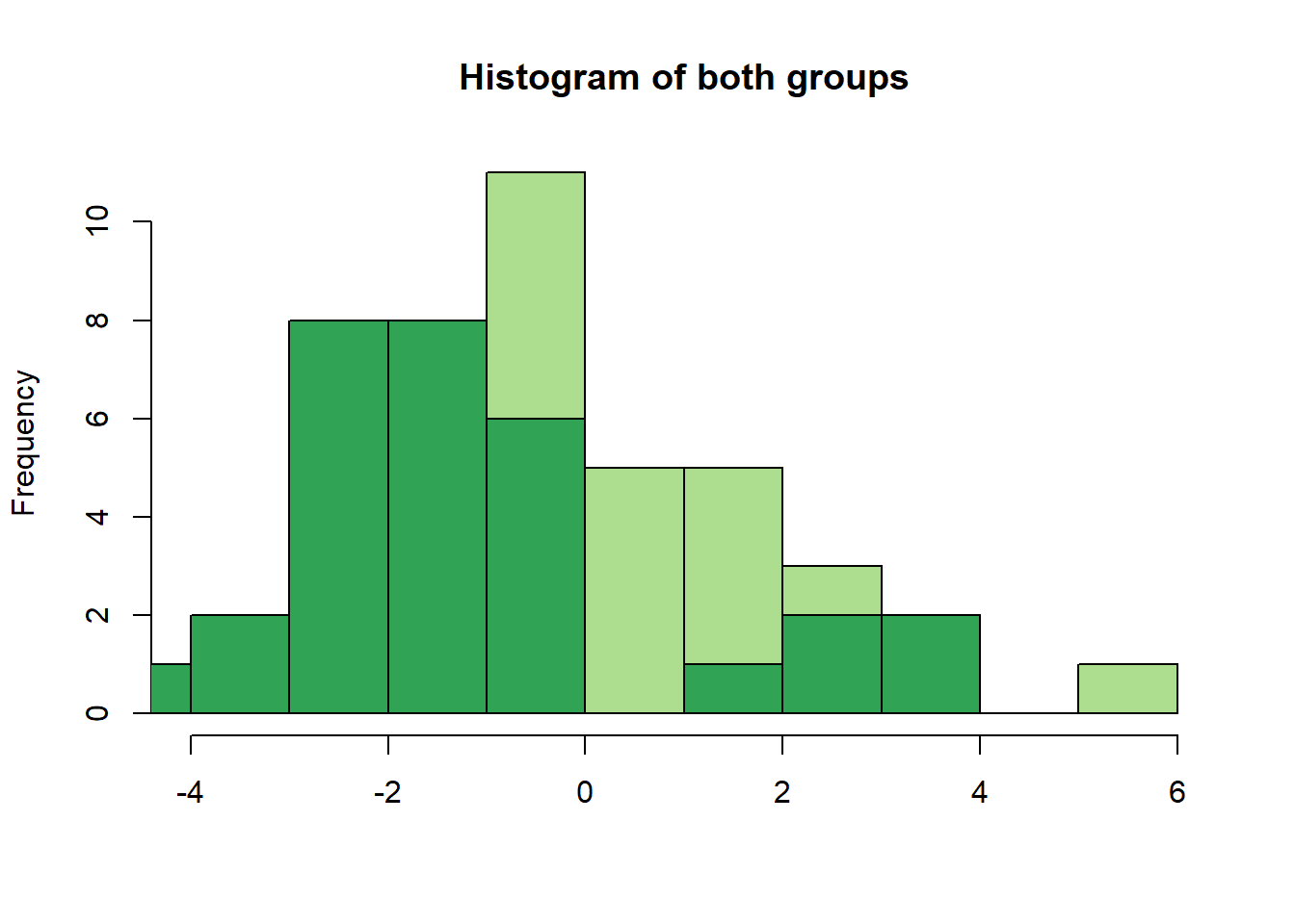
We can already make important observations from this plot:
We wanted to get normal distributions, but what we got here does not really look normal.
Why is that? Because we only have 30 people per group and taking only 30 values from the specified normal distributions does not really give us a good approximation of the real distribution.
This point is important: The sampling variability in such small groups is high and often, if small sample-studies (i.e. underpowered studies) find “effects”, they are often rather big and the consequence of this sampling variability rather than real differences of groups.
For example, by looking at the means of our sampled groups mean(group1) = 0.40715 and mean(group2) = -1.1032366 we see that the group mean of group 1 is actually closer to the mean that we specified for group 2 (i.e. 0) than to its own mean, while the mean for group 2 is far away from our intended mean.
Looking at the sds actually shows that they are quite close to what we wanted sd(group1) = 1.8059661 and sd(group2) = 1.9179992.
The \(Cohen's\ d\) that we wanted is also not presented very accurately at (mean(group1)-mean(group2))/(sqrt((sd(group1)^2+sd(group2)^2)/2)) = 0.8108043.
Again, if we would do this in Gpower, and specify a \(Cohen's\ d\), we will always work with an exact \(Cohen's\ d\), in a simulation approach we do not.
So let us run a t-test to see whether there is a significant difference here. First, we need to decide on an alpha-level again. What will we choose? Well, to have a good justification we have to elaborate on what the groups actually represent. Let us say that the difference between groups is related to an intervention that can elevate depressive symptoms. Thus, the control group (group1) did not get the intervention and scores higher on depressive symptoms while the treatment group (group2) is expected to score lower. Let us assume that this is the first study that we run and that, if we find anything we will follow it up by more extensive studies anyway. Therefore, we might not want to miss a possible effect by setting a too conservative alpha-level. If we find something in this study, we will conduct further studies in which we are more strict about the alpha level. Thus, we choose .10 for this first “pilot” study.
NOTE: The alpha-level “jusficications” in this tutorial are for educational purposes and to provide a starting point. They are obviously not as rigorous as we would like in a real research project. If you find yourself in a situation where you want to justify your alpha-level see Justify your alpha by Lakens et al. for a good discussion on this.
We can now run a t-test with R’s integrated t.test function.
t.test(group1, group2, paired = FALSE, var.equal = TRUE, conf.level = 0.9)##
## Two Sample t-test
##
## data: group1 and group2
## t = 3.1402, df = 58, p-value = 0.002656
## alternative hypothesis: true difference in means is not equal to 0
## 90 percent confidence interval:
## 0.7064042 2.3143690
## sample estimates:
## mean of x mean of y
## 0.407150 -1.103237The t-test shows, that this effect would be significant. However, we also got “lucky” and had a larger effect than we intended to have. To do a proper power analysis (lets say we first want to see whether 30 people per group are enough) we need to not only simulate each group once, but many many times and see how often we get a significant result at the desired alpha-level1. Moreover, we would like to have a power of at least 95%, again reflecting our view that we do not want to miss a possible effect.
In normal language these assumptions mean that if there is a difference, we will detect it in 19 out of 20 cases while, if there is no difference, we will only be incorrectly claiming that there is one in 1 out of 10 cases.
We will do this similarly to our simulations in part 1 of this tutorial.
set.seed(1)
n_sims <- 1000 # we want 1000 simulations
p_vals <- c()
for(i in 1:n_sims){
  group1 <- rnorm(30,1,2) # simulate group 1
  group2 <- rnorm(30,0,2) # simulate group 2
  p_vals[i] <- t.test(group1, group2, paired = FALSE, var.equal = TRUE, conf.level = 0.90)$p.value # run t-test and extract the p-value
}
mean(p_vals < .10) # check power (i.e. proportion of p-values that are smaller than alpha-level of .10)
## [1] 0.592Aha, so it appears that our power mean(p_vals < .10) = 0.592 is much lower than the 95% that we desired.
Thus, we did really get lucky in our example above when we found an effect of our intervention.
To actually do a legit power-analysis however, we would like to know how many people we do need for a power of 95 percent. Again we can modify the code above to take this into account.
set.seed(1)
n_sims <- 1000 # we want 1000 simulations
p_vals <- c()
power_at_n <- c(0) # this vector will contain the power for each sample-size (it needs the initial 0 for the while-loop to work)
cohens_ds <- c()
cohens_ds_at_n <- c()
n <- 30 # sample-size
i <- 2
while(power_at_n[i-1] < .95){
  for(sim in 1:n_sims){
    group1 <- rnorm(n,1,2) # simulate group 1
    group2 <- rnorm(n,0,2) # simulate group 2
    p_vals[sim] <- t.test(group1, group2, paired = FALSE, var.equal = TRUE, conf.level = 0.9)$p.value # run t-test and extract the p-value
    cohens_ds[sim] <- abs((mean(group1)-mean(group2))/(sqrt((sd(group1)^2+sd(group2)^2)/2))) # we also save the cohens ds that we observed in each simulation
  }
    power_at_n[i] <- mean(p_vals < .10) # check power (i.e. proportion of p-values that are smaller than alpha-level of .10)
    cohens_ds_at_n[i] <- mean(cohens_ds) # calculate means of cohens ds for each sample-size
    n <- n+1 # increase sample-size by 1
    i <- i+1 # increase index of the while-loop by 1 to save power and cohens d to vector
}
power_at_n <- power_at_n[-1] # delete first 0 from the vector
cohens_ds_at_n <- cohens_ds_at_n[-1] # delete first NA from the vector
The loop stopped at a sample-size of n-1 = 84 participants per group.
Thus make a conclusion about the effectiveness of our intervention at the specified alpha-level with the desired power we need 168 people in total.
To visualize the power we can plot it again, just as in the first part of the tutorial.
plot(30:(n-1), power_at_n, xlab = "Number of participants per group", ylab = "Power", ylim = c(0,1), axes = TRUE)
abline(h = .95, col = "red")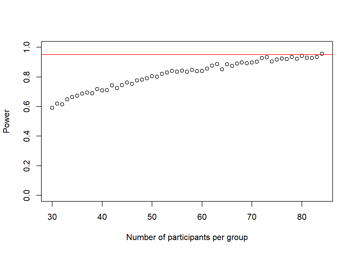
Again, this plot shows us how our power to detect the effect slowly increases if we increase the sample-size until it reaches our desired power.
There is another interesting observation to make here. In the code above, I also calculate the average \(Cohen's\ d\) for each sample size and the plot below shows how it changes with increasing sample-size.
plot(30:(n-1), cohens_ds_at_n, xlab = "Number of participants per group", ylab = "Cohens D", ylim = c(0.45,0.55), axes = TRUE)
abline(h = .50, col = "red")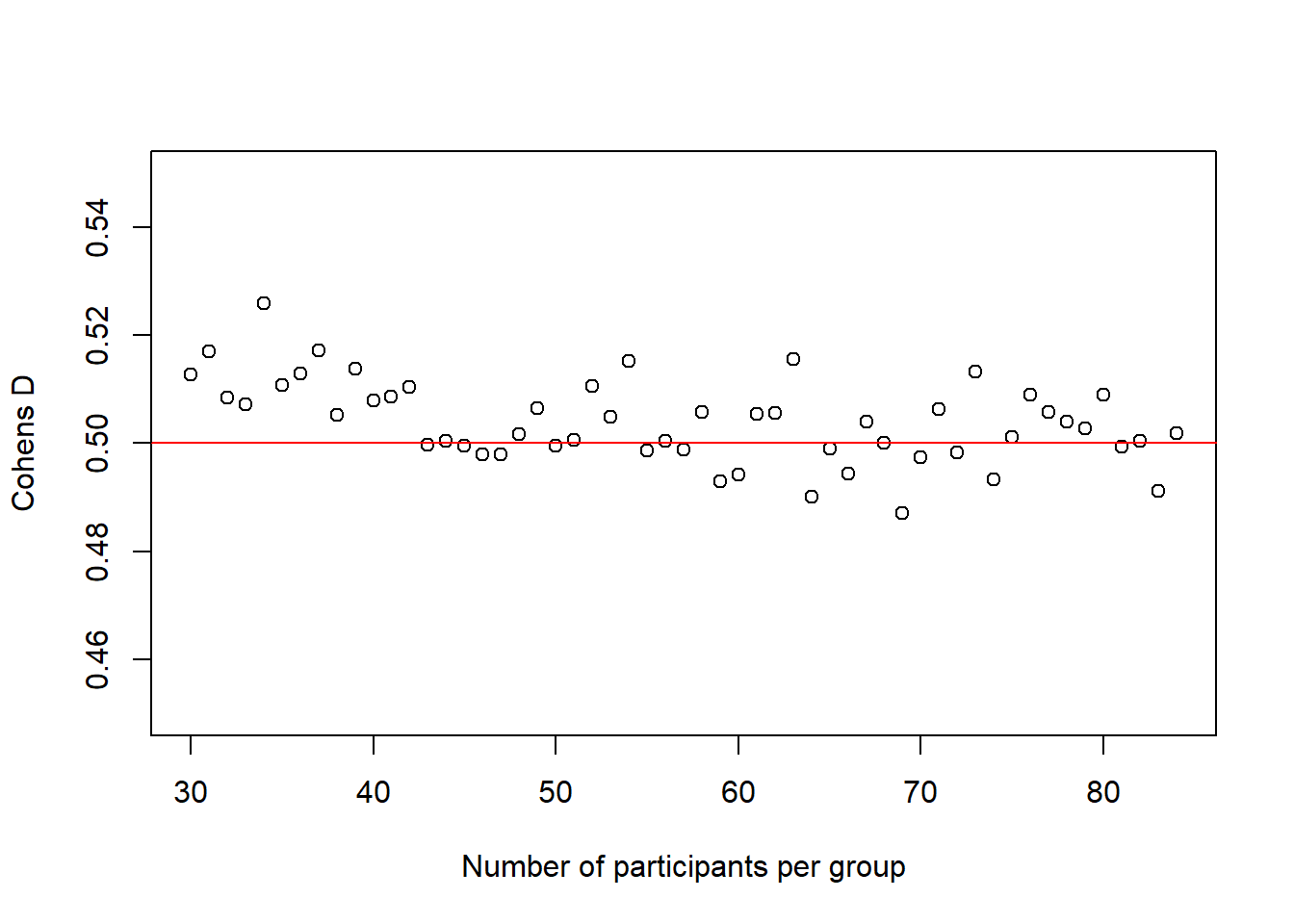
It is not super obvious in this plot and I had to change the scale of the y-axis quite a bit to make it visible, but we can actually see how our average \(Cohen's\ d\) initially deviates slightly more from the desired \(Cohen's\ d\) of .50 than in de end. In other words, in the beginning, for small sample-sizes there is more fluctuation than for bigger sample-sizes. That is pretty neat, as it seems very desirable that a power-estimation procedure takes into account that for smaller sample-sizes, even if the effect in the population is exactly the same (i.e. we always sample groups with a difference of \(Cohen's\ d\) = .50) it is just less precise.
Let’s have a brief summary of what we did so far. We just used the formula for \(Cohen's\ d\) to give our groups a certain difference that we are interested in, ran 1000 simulated experiments for each sample-size and calculated the power, just as in the first part of the tutorial.
However, I want to mention again that, even though it is convenient to specify the effect-size this way as it saves us from having to specify precise group means and standard-deviations directy and makes the specification more comparable, it is often preferable to specify the parameters on the original scale that we are interested in. This is especially the case if we have previous data on a research topic that we can make use of. Moreover, for more complex designs with many parameters, standardized effect sizes are often difficult to obtain and we are forced to make our assumptions on the original scale of the data. We will see this in later examples.
Simulating a within-subject t-test
Intuitively, it might seem that we can use the exact same approach above for a paired t-test as well. However, the problem with this is that in a paired t-test we get 2 data-points from the same individual. For example, image we have a group of people that get an intervention and we measure their score before and after the intervention and want to compare them with a paired t-test. In this case, the score of the post-measure of a given individual is not completely independent of the score of the pre-measure. In other words, somebody who scores very low on the pre-measure will most likely not score very high on the post-measure and vice versa.
Thus, there is a correlation between the pre- and the post-measures in that the pre-measures already tell us a little bit about what we can expect on the post-measure. You probably already knew this but why does this matter for power simulation, you might wonder. It matters as it directly influences our power to detect an effect as we will see later. For now let’s just keep in mind that it is important.
So what do we do in a situation with correlated data as in the pre-post intervention situation? There are two ways we can go from here. First, we can simulate correlated normal distributions, as already mentioned above. However, for the particular case of a paired sample t-test, we can also just make use of the fact that, in the end, we are testing whether the difference between post- and pre-measures is different from 0. In this case, the correlation between the pre and the post-measure is implicitely handled when substracting the two measures. This way, we do not need to directly specify it. If the correlation is close to one, the standard-deviation of the difference scores will be very small, if it is zero, we will end up with the same situation that we have in the independent-sample t-test. Thus, we can just make use of a one-sample in which we test whether the distribution of difference-scores differs from zero as the paired t-test is equivalent to the one-sample t-test on difference scores (see Lakens, 2013 for more details on this).
Though the one-sample approach is easier to simulate, I will describe both approaches in the following as the first approach (simulating correlated normal-distributions) is more flexible and we need it for the situations we deal with later.
Using a one-sample t-test approach
When we want to do our power-calculation based on the one-sample t-test approach, we only have to specify a single difference-score distribution. We can do this again, based on the \(Cohen's\ d\) formula, this time for a one-sample scenario:
\[ Cohen's\ d = \frac{M_{diff} - \mu_0}{SD_{diff}}\]
In the above formula, to get our values for the simulation we can substitute the \(\mu_0\) by 0 (as our null-hypothesis is no difference) and solve the equation in the same way as above by fixing the mean-difference between pre- and post-measure, \(M_{diff}\) to 1 and calculating the sd we need for each given \(Cohen's\ d\), for instance
\[ 0.5 = \frac{1}{SD_{diff}}\]
putting this into Rs solve function again, we unsurprisingly get a 2 in this case.
solve(0.5, 1)## [1] 2To run our simulation we just need to modify the code above to run a one-sample t-test rather than a two-sample t-test and change the formula for \(Cohen's\ d\)
set.seed(1)
n_sims <- 1000 # we want 1000 simulations
p_vals <- c()
power_at_n <- c(0) # this vector will contain the power for each sample-size (it needs the initial 0 for the while-loop to work)
cohens_ds <- c()
cohens_ds_at_n <- c()
n <- 2 # sample-size
i <- 2
while(power_at_n[i-1] < .95){
  for(sim in 1:n_sims){
    difference <- rnorm(n,1,2) # simulate the difference score distribution
    p_vals[sim] <- t.test(difference, mu = 0, conf.level = 0.90)$p.value # run t-test and extract the p-value
    cohens_ds[sim] <- mean(difference)/sd(difference) # we also save the cohens ds that we observed in each simulation
  }
    power_at_n[i] <- mean(p_vals < .10) # check power (i.e. proportion of p-values that are smaller than alpha-level of .10)
    cohens_ds_at_n[i] <- mean(cohens_ds) # calculate means of cohens ds for each sample-size
    n <- n+1 # increase sample-size by 1
    i <- i+1 # increase index of the while-loop by 1 to save power and cohens d to vector
}
power_at_n <- power_at_n[-1] # delete first 0 from the vector
cohens_ds_at_n <- cohens_ds_at_n[-1] # delete first NA from the vector
We see that the loop stopped at n = 43 so the sample size we need is n-1 = 42
We can plot the power-curve again
plot(2:(n-1), power_at_n, xlab = "Number of participants per group", ylab = "Power", ylim = c(0,1), axes = TRUE)
abline(h = .95, col = "red")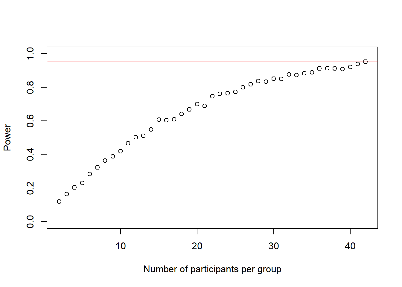
and the \(Cohen's\ d\) values:
plot(2:(n-1), cohens_ds_at_n, xlab = "Number of participants per group", ylab = "Cohens D", ylim = c(0.0,1.0), axes = TRUE)
abline(h = .50, col = "red")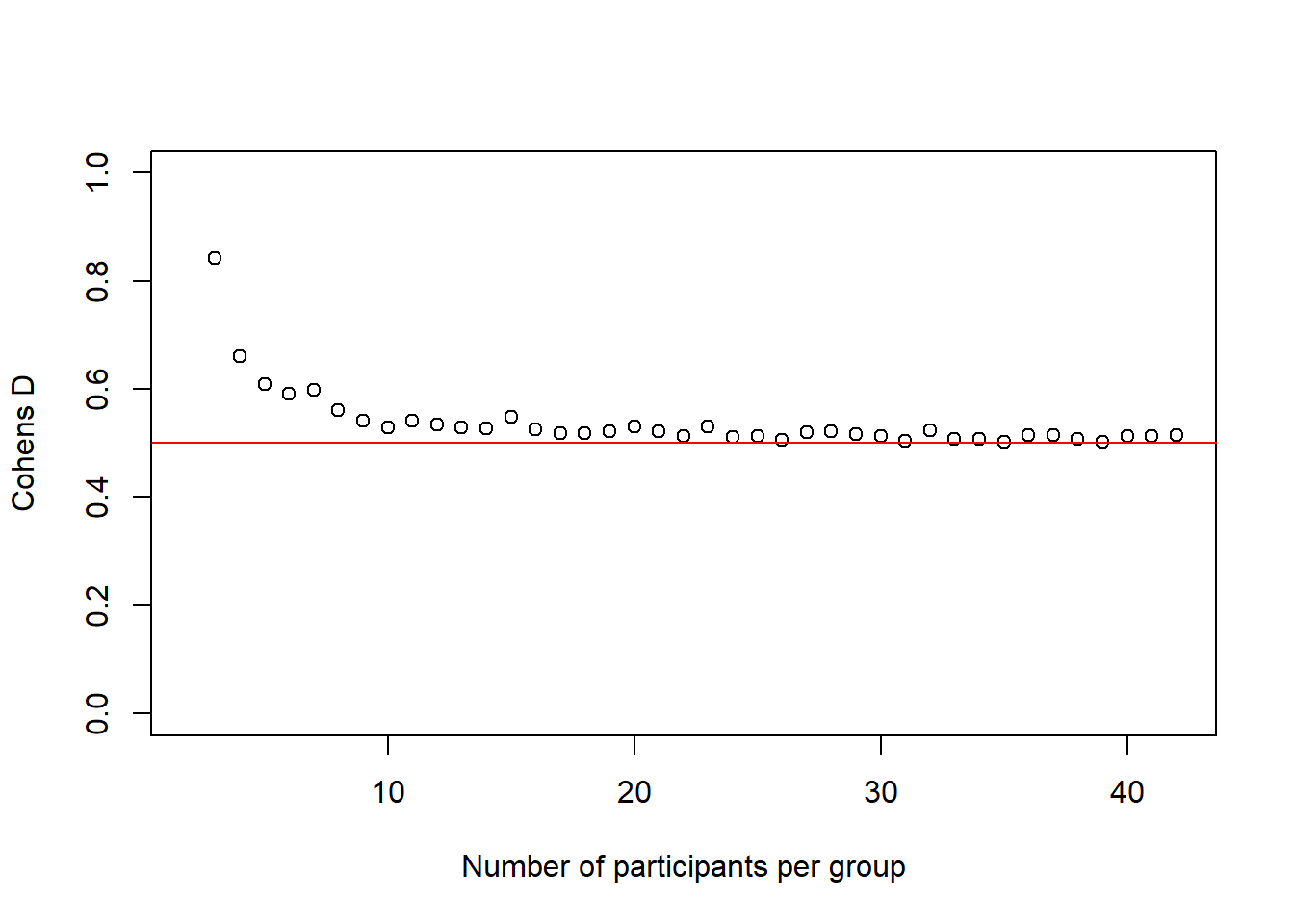
We see again, and this time more dramatically, how our simulated effect size becomes more accurate the bigger our sample gets.
Using a correlated-samples paired t-test approach
The relationship between \(SD_{diff}\) and the correlation
In the above example, we respecified a paired t-test as a one-sample t-test on the difference scores. However, what we are actually working with is two correlated distributions of measurements. To demonstrate this point, let us have a look at how we would actually calculate the standard deviation of the difference scores (\(SD_{diff}\)) in the above equation for \(Cohen's\ d\). The formula to calculate \(SD_{diff}\) from the standard deviation of the two measurements (pre and post) and their correlation is:
\[SD_{diff} = \sqrt{SD_{pre}^2+SD_{post}^2-2r \times SD_{pre} \times SD_{post}} \]
It is not important at this point to understand why this is the case (we will just trust Cohen on this) but see how we can, for any given \(SD_{diff}\) and assuming both groups have, for example, a standard deviation of 2, solve the formula to see what correlation (the \(r\) in the above formula) it would imply.
Imagine, for instance, we assume (like in the independent-samples t-test above) that both measures have a standard-deviation of 2 and that the standard-deviation of the difference scores would also be 2 so that we would have the same situation as in the one-sample t-test example above, where we had a mean-difference of 1 and a difference-score standard-deviation of 2.
Filling this in we get
\[2 = \sqrt{2^2+2^2-2r \times 2 \times 2} \]
Solving this equation for \(r\), we get2 \(r = 0.5\):
Therefore, interestingly the situation in which we use the same groups as above and assume that we would get the same \(SD_{diff}\) of 2 as we assumed in our one-sample situation would imply that the correlation between the pre- and the post-measure is \(r = 0.5\). What does this mean? Well, lets see what happens if we assume a correlation of \(r = .90\) and see what \(SD_{diff}\) we get:
\[SD_{diff} = \sqrt{2^2+2^2-2 \times 0.90 \times 2 \times 2} \]
Solving this in R gives us: sqrt(2^2+2^2-2*0.9*2*2) = 0.89.
Thus, if the correlation increases the standard-deviation of the difference-scores becomes smaller.
If we do the same with a correlation of .10 we get sqrt(2^2+2^2-2*0.1*2*2) = 2.68.
Thus, when the correlation decreases the standard-deviation becomes bigger.
Interestingly, this demonstrates that for the same mean-difference, a high correlation results in a larger \(Cohen's\ d\) as calculated for the difference scores in the one-sample case.
In other words, as the pre-scores tend to be more similar to the post-scores (i.e. they have a high correlation), the standard-deviation of the difference scores decreases.
This, in turn, results in higher power to detect an effect.
To sum up all of the above, we can either specify a difference-score distribution directly and thereby imply a certain correlation by specifying the \(SD_{diff}\), or we can see what \(SD_{diff}\) we get with a certain correlation by using the formula above and use the result for the one-sample simulation.
However, instead of working with the one-sample t-test, in the next section, we will see how we can directly simulate correlated normal-distributions in R.
Simulating correlated normal-distributions and demystifying the multivariate normal.
In real life, almost everything is correlated to some degree. Though these correlations are often not of interest, they sometimes are and in a good simulation we want to acknowledge them. For instance, predictors in a regression might be correlated or random effects in a mixed-model.
The following part is (again) longer than I intended but I feel that it is important to understand how we simulate correlated normal-distributions and what a multivariate normal-distribution is. In most cases later on we will deal with some kind of correlated normal distributions (in mixed-models we will always encounter them for example) so I think it helps if we have a look at them now in an easier example, so we have one problem less to worry about later on.
Rephrasing the problem of simulating two correlated normal-distributions, we can say that we want to simulate a multivariate normal distribution or, more specifically in this case, a bivariate normal distribution.
If you never heard these terms before, they might seem very opague, so let’s see what they are.
I will first show how we can simulate them, and explain what exactly this multivariate normal distribution means afterwards with a little visual intuiton.
We can simulate a multivariate normal distribution by using the mvrnorm() function from the MASS package but it works slightly different than the simulation functions that we have used so far (rnorm and rbinom).
Lets have a look at how this works (code explained below).
require(MASS) # load MASS package## Loading required package: MASSpre_post_means <- c(pre = 0,post = 1) # define means of pre and post in a vector
pre_sd <- 2 # define sd of pre-measure
post_sd <- 2 # define sd of post-measure
correlation <- 0.5 # define their correlation
sigma <- matrix(c(pre_sd^2, pre_sd*post_sd*correlation, pre_sd*post_sd*correlation, post_sd^2), ncol = 2) # define variance-covariance matrix
set.seed(1)
bivnorm <- data.frame(mvrnorm(10000, pre_post_means, sigma)) # simulate bivariate normalThe above code samples 10,000 observations from a bivariate normal-distribution, or in terms of our example, it samples 10,000 pre-measures with 10,000 correlated post-measures.
The first thing that is different from our earlier simulations is the first line of the code pre_post_means <- c(0,1).
Instead of defining our means seperately for each measurement, as we have done earlier in the independent-sample case, we now put the pre- and post-measurement mean that we assume into a vector.
This is because we will simulate both measurements together in the mvrnorm function, and therefore both means need to be provided at the same time.
Secondly, we define the standard-deviations of both measurements just as we did earlier and also specify a correlation that we would like our data-points to have, in this case 0.5.
Now, the line matrix(c(pre_sd^2, pre_sd*post_sd*correlation, pre_sd*post_sd*correlation, post_sd^2), ncol = 2) does something that we have not done before and it might look quite confusing.
What we are doing here is specifying the variance-covariance matrix.
This is nothing more than a table containing the variances of our pre- and post-measurement (the first and the last entry in the list) and the covariance between the two variables twice - once for each measurement (the middle 2 entries in the list).
Conceptually you can see this variance-covariance matrix as the standard-deviation of the multivariate normal that mvrnorm needs instead of the standard-deviation that we put into rnorm earlier.
We can visualize the variance-covariance matrix sigma to demystify it a bit.
colnames(sigma) <- c("pre", "post")
rownames(sigma) <- c("pre", "post")
sigma
## pre post
## pre 4 2
## post 2 4Thus, this matrix is nothing more than a table containing the variance of each variable (4 in each case) and their covariance (i.e. the correlation of the two multiplied by both standard-deviations (\(Cov(pre,post) = \rho(pre,post)*sd_{pre}*sd_{post}\)).
In the next line of the code we put this all into mvrnorm to simulate our bivariate normal distribution and store the results in a data-frame with 2 columns, each containing one measurement point:
head(bivnorm)## pre post
## 1 -0.2807182 -0.8893814
## 2 1.3746052 0.2615539
## 3 -0.4119554 -1.4827470
## 4 3.9486678 2.5775470
## 5 1.0711637 1.0702847
## 6 -0.8961042 -0.9460816When we run cor(bivnorm$pre, bivnorm$post) we see that indeed their correlation is 0.52 and close to what we specified.
To see how we can imagine such a bivariate normal distribution, we can visualize it the following way.
If we draw a histogram of each measurement individually, it looks like this.
par(mfrow=c(1,2))
hist(bivnorm$pre, main = "pre-measure")
hist(bivnorm$post, main = "post-measure")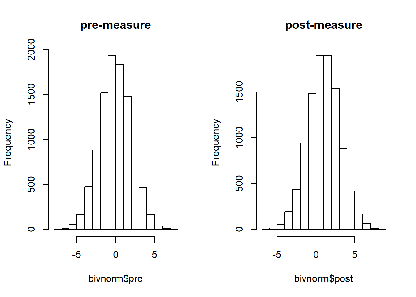
However, imagine we would not only look at each histogram seperately but we would combine them into one plot by putting the pre-measure scores of each simulated individual on the x-axis and putting the post-measures on the y-axis like this:
plot(bivnorm$pre, bivnorm$post, xlab = "pre-measure", ylab = "post-measure")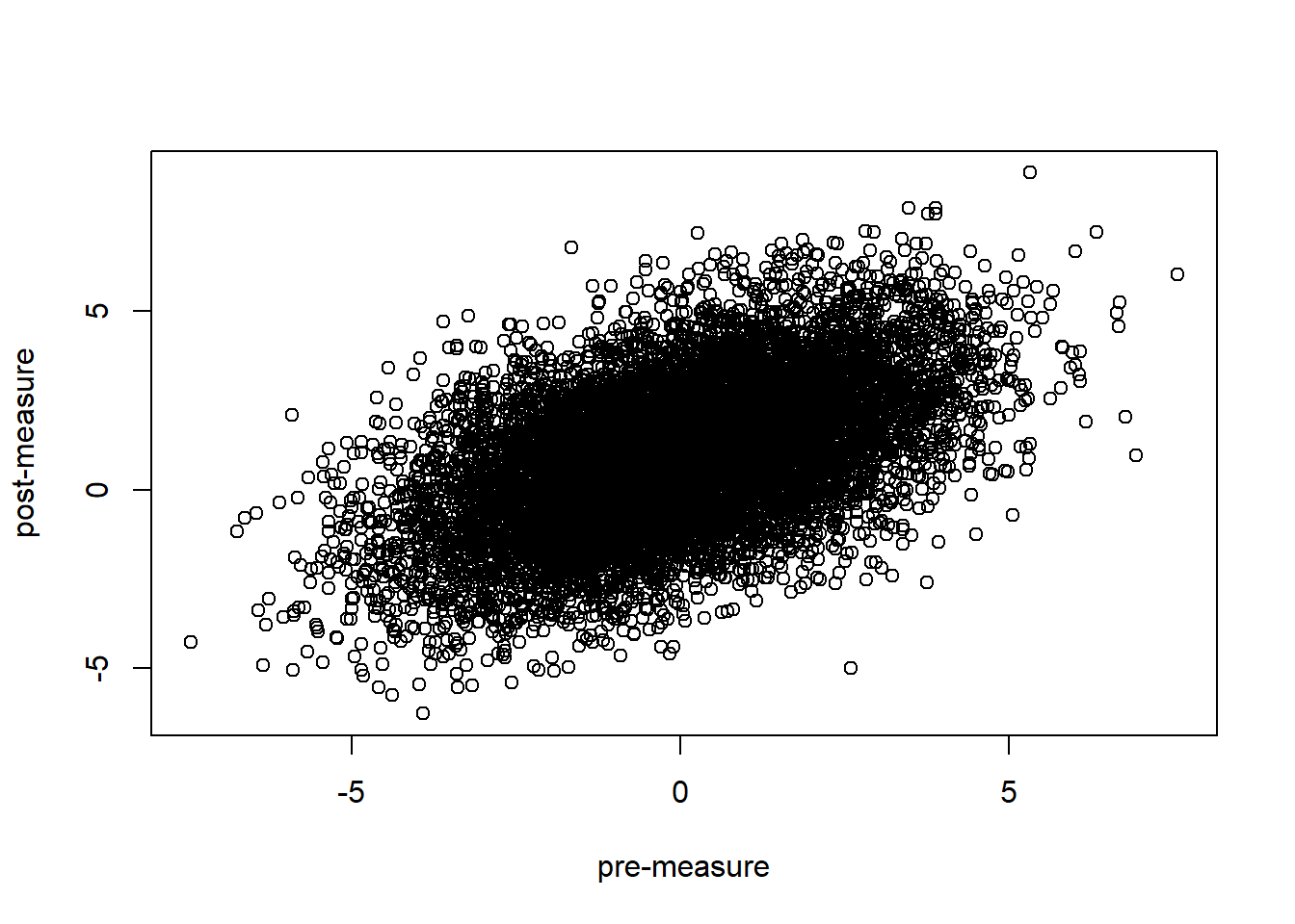
In the above plot, we can clearly see the correlations between the two measurements that we put in the data. More elegantly, we can combine the two histograms in the following way.
bivnorm_kde <- kde2d(bivnorm[,1], bivnorm[,2], n = 50) # calculate kernel density (i.e. the "height of the cone on the z-axis"; not so important to understand here)
par(mar = c(0, 0, 0, 0)) # tel r not to leave so much space around the plot
persp(bivnorm_kde, phi = 45, theta = 30, xlab = "pre-measure", ylab = "post-measure", zlab = "frequency") # plot the bivariate normal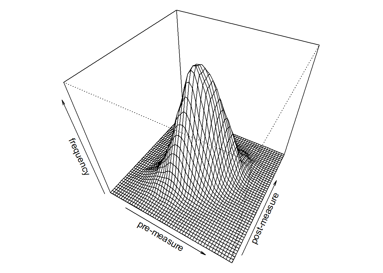
Here, we see clearly how our bivariate normal distribution is nothing more than the 2 normal-distributions of each measurement-point combined into one “cone-shaped” normal distribution that has a certain correlation.
The plot below shows how this cone looks with different correlations.
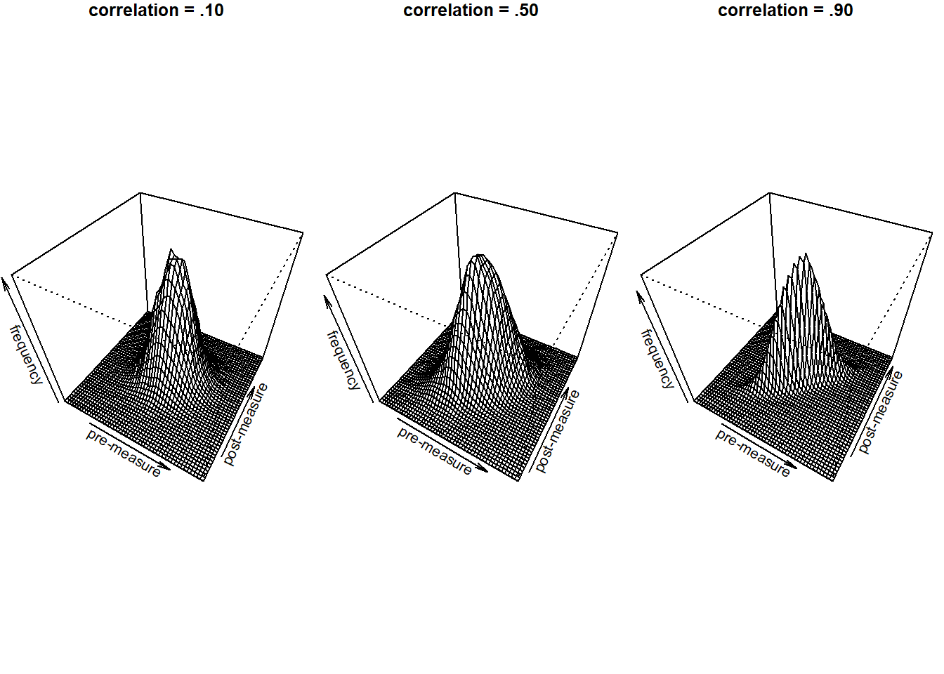
Notice how for higher correlations, the cone becomes more and more narrow and starts looking like a “shark-fin” with a correlation of .90. This “narrowring” of the cone is the visualization of why the standard-deviations of the difference scores get more narrow.
If we visualize this as a point cloud again the three correlations look like this:
bivnorm_10 <- as.data.frame(bivnorm_10)
bivnorm_90 <- as.data.frame(bivnorm_90)
par(mfrow = c(1,3))
plot(bivnorm_10$pre, bivnorm_10$post)
plot(bivnorm$pre, bivnorm$post)
plot(bivnorm_90$pre, bivnorm_90$post)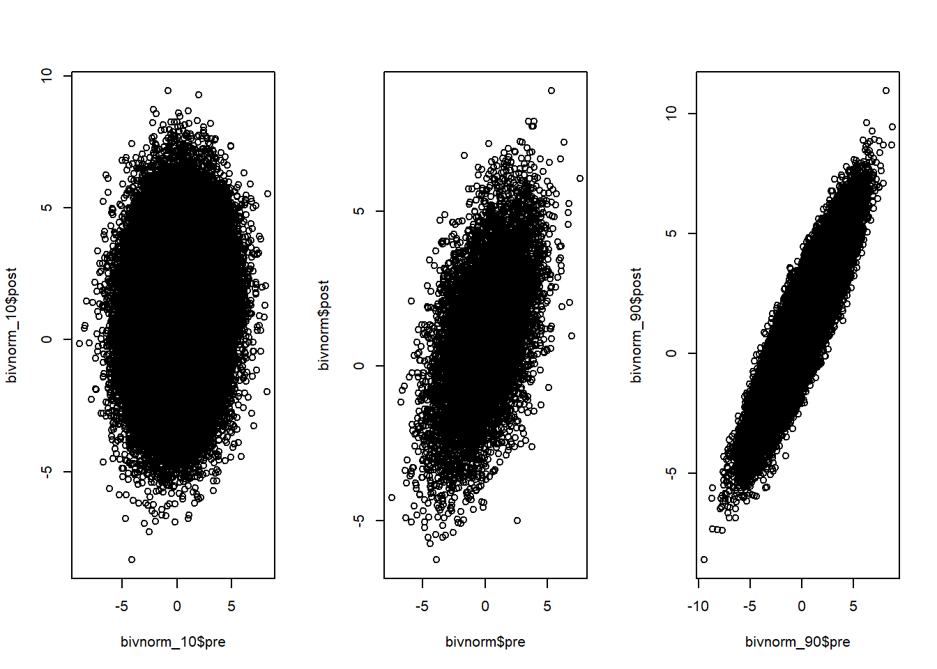
This again, clearly shows the manipulatino between the pre- and post measures.
Power-analysis with the multivariate normal
Now that we know what we are doing when using mvrnorm we can go ahead and do a power-simulation for the example above with a bivariate normal-distribution.
However, as we are not sure how big our correlation is, we can try 3 different correlations in the code above by placing the simulation in another for-loop and telling it to try different correlations.
mu_pre_post <- c(pre = 0, post = 1)
sd_pre <- 2
sd_post <- 2
correlations <- c(0.1, 0.5, 0.9)

set.seed(1)
n_sims <- 1000 # we want 1000 simulations
p_vals <- c()
# this vector will contain the power for each sample-size (it needs the initial 0 for the while-loop to work)
cohens_ds <- c()

powers_at_cor <- list()
cohens_ds_at_cor <- list()

for(icor in 1:length(correlations)){ # do a power-simulation for each specified simulation
  n <- 2 # sample-size
  i <- 2 # index of the while loop for saving things into the right place in the lists
  power_at_n <- c(0)
  cohens_ds_at_n <- c()
  sigma <- matrix(c(sd_pre^2, sd_pre*sd_post*correlations[icor], sd_pre*sd_post*correlations[icor], sd_post^2), ncol = 2) #var-covar matrix
  while(power_at_n[i-1] < .95){
    for(sim in 1:n_sims){
      bivnorm <- data.frame(mvrnorm(n, mu_pre_post, sigma)) # simulate the bivariate normal
      p_vals[sim] <- t.test(bivnorm$pre, bivnorm$post, paired = TRUE, var.equal = TRUE, conf.level = 0.9)$p.value # run t-test and extract the p-value
      cohens_ds[sim] <- abs((mean(bivnorm$pre)-mean(bivnorm$post))/(sqrt(sd(bivnorm$pre)^2+sd(bivnorm$post)^2-2*cor(bivnorm$pre, bivnorm$post)*sd(bivnorm$pre)*sd(bivnorm$post)))) # we also save the cohens ds that we observed in each simulation
    }
    power_at_n[i] <- mean(p_vals < .10) # check power (i.e. proportion of p-values that are smaller than alpha-level of .10)
    names(power_at_n)[i] <- n
    cohens_ds_at_n[i] <- mean(cohens_ds) # calculate means of cohens ds for each sample-size
    names(cohens_ds_at_n)[i] <- n
    n <- n+1 # increase sample-size by 1
    i <- i+1 # increase index of the while-loop by 1 to save power and cohens d to vector
  }
  power_at_n <- power_at_n[-1] # delete first 0 from the vector
  cohens_ds_at_n <- cohens_ds_at_n[-1] # delete first NA from the vector
  powers_at_cor[[icor]] <- power_at_n # store the entire power curve for this correlation in a list
  cohens_ds_at_cor[[icor]] <- cohens_ds_at_n # do the same for cohens d
  names(powers_at_cor)[[icor]] <- correlations[icor] # name the power-curve in the list according to the tested correlation
  names(cohens_ds_at_cor)[[icor]] <- correlations[icor] # same for cohens d
}
Again, the above code runs a power-simulation, or more specifically three power-analyses, one for each correlation that we wanted to test.
Notice how this time we specify paired = TRUE in the t.test function, to indicate that we are dealing with non-independent observations.
Also note that a new part of the code saves the power_at_n vector to a list called power_at_cor.
This list, will have 3 elements, each of them the power curve for one of the correlations.
We can access each power-curve bei either powers_at_cor[[1]] to get the first vector in the list (the double square brackets mean first entire vector rather than first number only) or we can use it by indicating its name as powers_at_cor$0.1` to tell R that we want the power curve for a correlation of .10.
We can plot these power-curves next to each other
par(mfrow=c(1,3))
plot(2:(length(powers_at_cor$`0.1`)+1), powers_at_cor$`0.1`, xlab = "Number of participants", ylab = "Power", ylim = c(0,1), axes = TRUE, main = "correlation = 0.1")
abline(h = .95, col = "red")
plot(2:(length(powers_at_cor$`0.5`)+1), powers_at_cor$`0.5`, xlab = "Number of participants", ylab = "Power", ylim = c(0,1), axes = TRUE, main = "correlation = 0.5")
abline(h = .95, col = "red")
plot(2:(length(powers_at_cor$`0.9`)+1), powers_at_cor$`0.9`, xlab = "Number of participants", ylab = "Power", ylim = c(0,1), axes = TRUE, main = "correlation = 0.9")
abline(h = .95, col = "red")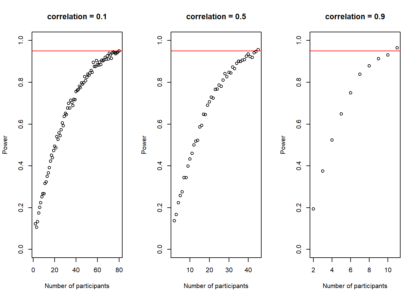
Here we see how drastically the correlation influences the power in this situation. With a high correlation, we need only very few participants to achieve the desired power in the specified case. Why is this? The reason for this is what we had a look at above: The decreasing standard-deviation of the difference scores the higher the correlation gets.
This is how the effect-sizes look.
par(mfrow=c(1,3))
plot(2:(length(cohens_ds_at_cor$`0.1`)+1), cohens_ds_at_cor$`0.1`, xlab = "Number of participants", ylab = "Cohens D", ylim = c(0,1), axes = TRUE, main = "correlation = 0.1")
abline(h = .50, col = "red")
plot(2:(length(cohens_ds_at_cor$`0.5`)+1), cohens_ds_at_cor$`0.5`, xlab = "Number of participants", ylab = "Cohens D", ylim = c(0,1), axes = TRUE, main = "correlation = 0.5")
abline(h = .50, col = "red")
plot(2:(length(cohens_ds_at_cor$`0.9`)+1), cohens_ds_at_cor$`0.9`, xlab = "Number of participants", ylab = "Cohens D", ylim = c(0,10), axes = TRUE, main = "correlation = 0.9")
abline(h = .50, col = "red")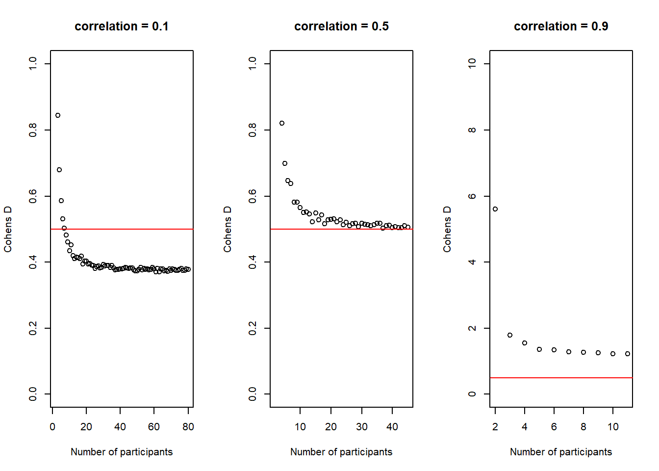
For .10 the value of the effect-size seems slightly underestimated, for .50 it approaches .50 just as in the two-sample case and for .90 it seems overestimated by quite a bit. Did something go wrong? Well no. As we’ve seen above \(Cohen's\ d\) is calculated by dividing the mean-difference by the standard-deviation of the difference scores which becomes smaller and smaller with increasing correlation. Therefore, calculated this way, \(Cohen's\ d\) is much bigger in the case with the larger correlation. This is also why we seem to have much bigger power - we just work with a larger effect size than we intended. We can even calculate by how much the effect-size is influenced by the correlation by dividing the effect-size that we would calculate based on the means and sds of our groups by \(\sqrt{2(1-r)}\).
r = .90 –> 0.5/sqrt(2*(1-.90)) = 1.118034
r = .50 –> 0.5/sqrt(2*(1-.50)) = 0.5
r = .10 –> 0.5/sqrt(2*(1-.10)) = 0.372678
You might wonder how we can specify effect-sizes in these cases of correlated data. Do we “correct” the expected effect for the correlation or do we just assume that it is .50 and use the one-sample scenario above? I do not have a good answer for this. In many cases it might be fine to only specify the effect-size of the pre-post design based on the difference scores as we did in the one-sample case. In some cases, however, we might find the correlation very important or have more information about the correlation of 2 measures than about the change in measures due to an intervention. In those cases, it might make sense to be very specific about the expected correlations and be aware that we might need more data if the correlation is low. Eventually, our data stem from an underlying data generating process that includes the correlation between variables and measures and it is always good to be aware of the factors that might possibly influence the results. When we collect data in a pre-post design, we do in fact measure a score at 2 time-points and do not directly assess the difference. When we specify the standard-deviation of the difference scores however, to arrive at a given \(Cohen's\ d\), we implicitely make assumptions about the correlations of these two measures.
The Take-home message here is that correlations matter and that we need to be aware of this. The good news is that power-simulations will at least make us aware of these factors and show us how different assumptions lead to different results.
Summary: Our first simulations with t-tests
This was the last bit that I wanted to discuss about simulating t-tests and the end of part II of this tutorial.
We have now learned how to simulate a t-test by using either \(Cohen's\ d\) as an effect-size estimate and, if necessary, tell R that our two groups, or measurements, are correlated in some way.
What we learned above is not restricted to doing t-tests however.
Simulating univariate (i.e. uncorrelated) or multivariate (i.e. correlated) normal-distributions will be what we do most of the time in part III and part IV of the tutorial.
The only thing that will change for more complicated designs is how we combine the different tools that we learned in this part to achieve our goal.
In part III of this tutorial, we will see how we can basically run every analysis as a linear model using the lm function instead of using the t.test function for t-tests, the aov function for ANOVA-designs and so forth.
By exploring how this works for t-test, anova and regression we will simulate our way through the third part and be flexible enough to simulate any classical research designs that we would, for example, be able to do in GPower. In part IV we will go beyond this and simulate mixed-effect models.
Footnotes
Think back to the possible sequences of coin tosses in part I. Instead of possible sequences of coin-tosses, we deal with possible sequences of people-scores here, assuming that they come from the underlying distribution that we specify. To get a good approximation of all the possible samples that we could get that still follow the specified distribution, we need to simulate many, many times.↩︎
This is how we solve for r:↩︎